Ordinary differential equation

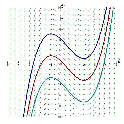
Possible solutions to the differential equation $\frac{dy}{dx}=x^2-x-2$ represented by a slope field.

An ordinary differential equation or ODE (as opposed to a partial differential equation) is a type of differential equation that involves a function of only one independent variable. It can simply be defined, for a layman, as any equation that involves any combination of the following:

• An independent variable ($x$)
• Functions of the independent variable (or dependent variables) ($g(x)$)
• A primary dependent variable (the function in question) ($y(x)$)
• And, necessarily, any number of and degrees of derivatives of the primary function (${\frac {dy}{dx}},{\frac {d^{2}y}{dx^{2}}}$)

An example differential equation is as follows:

$x^{2}y+3{\frac {d^{2}y}{dx^{2}}}-xy{\frac {d^{2}y}{dx^{2}}}=3$

Methods of solving

First order

See also: Euler's method

First order first degree differential equations in the form

${\frac {dy}{dx}}=f(x)$

Can be solved with direct integration.

Separable equations

Main article: Separable differential equation

Separable equations are the one of the easiest to solve. For any ODE in the form

$\frac{dy}{dx}=f(x)g(y)$

the solution is

$\int {\frac {dy}{g(y)}}=\int f(x)dx$

General linear equations

Main article: Linear differential equation

For linear equations in the form

$\frac{dy}{dx} + f(x)y = g(x)$,

the solution can be found with the formula

$y={\frac {1}{\mu }}\left(\int \mu g(x)dx+C\right),\,\,\mu =e^{\int f(x)dx}$

Bernoulli equations

Main article: Bernoulli differential equation

Bernoulli differential equations are those in the form

${\frac {dy}{dx}}+f(x)y=g(x)y^{n}$,

They can be solved by transforming them into linear differential equations by substituting.

Exact equations

Main article: Exact differential equation

Exact differential equations are those in the form

$m(x,y)dx+n(x,y)dy=0\,\,{\text{if}}\,\,{\frac {\partial }{\partial y}}m(x,y)={\frac {\partial }{\partial x}}n(x,y)$

and will have the solution

$\int m(x,y)dx+\int n(x,y)dy=C$

Systems of differential equations

By viewing the matrix A as a linear transformation, one can create a vector field called the phase portrait based on the mapping from x (the vector representing a given point) to x', similarly to a slope field. This particular phase portrait is based on the equation ${\tfrac {d^{2}y}{dt^{2}}}+(y^{2}-1){\tfrac {dy}{dt}}+y=0.$

A system of ODEs in the form

${\begin{bmatrix}x'_{1}\\\vdots \\x'_{n}\end{bmatrix}}={\begin{bmatrix}C_{11}&\cdots &C_{1n}\\\vdots &\ddots &\vdots \\C_{n1}&\cdots &C_{nn}\end{bmatrix}}{\begin{bmatrix}x_{1}\\\vdots \\x_{n}\end{bmatrix}}$

or, in more compact notation,

${\vec {x}}'=A{\vec {x}}$

the general solution will be

${\vec {x}}=C_{1}{\vec {v}}_{1}e^{\lambda _{1}t}+\cdots +C_{n}{\vec {v}}_{n}e^{\lambda _{n}t}$

where $\vec{v}$ and $\lambda$ represent the eigenvectors and eigenvalues of A, respectively. Higher order differential equations can be converted into such a system by making the substitution

$x_{n}=y^{(n)}(t)$

differentiating, and substituting variables from the original equation for derivatives of y to yield a system of first order ODEs. For example:

$y''-2y'+y=0$

We can make the substition

${\begin{bmatrix}x_{1}\\x_{2}\end{bmatrix}}={\begin{bmatrix}y\\y'\end{bmatrix}}$

${\begin{bmatrix}x_{1}\\x_{2}\end{bmatrix}}'={\begin{bmatrix}y'\\y''\end{bmatrix}}={\begin{bmatrix}x_{2}\\2x_{2}-x_{1}\end{bmatrix}}$

${\vec {x}}'={\begin{bmatrix}0&1\\2&-1\end{bmatrix}}{\vec {x}}$

Higher order equations

See also: Laplace transform

In general, if f(x) and g(x) are both solutions to a differential equation, C₁f(x) + C₂g(x) is also a solution.

Homogenous equations

$a{\frac {d^{2}y}{dx^{2}}}+b{\frac {dy}{dx}}+cy=0$

Differential equations in this form can be solved by first finding the roots of the auxiliary or characteristic equation, which is equal to

$ar^{2}+br+c=0$

The roots may be real or complex. If the roots are $r_{1}, r_{2}$ then the general solution will be:

$y=C_{1}e^{r_{1}x}+C_{2}e^{r_{2}x}$

If the characteristic equation has only one solution, the general solution of the ODE will be

$y=C_{1}e^{rx}+C_{2}xe^{rx}$

If the roots are complex and equal to $a\pm bi$, by Euler's formula the solution simplifies to

$y=e^{ax}(C_{1}\cos(bx)+C_{2}\sin(bx))$

The constant of integration is not restricted to real numbers in this case.

Method of undetermined coefficients

This method is used to find a particular solution for non-homogeneous equations by using a similar function as a potential particular solution Y_P and adjusting the coefficients. It is especially useful when the forcing term is a polynomial, trigonometric function, or exponential function, however if there is information known about the particular integral required different guesses can be tried.

For example:

$y''+3y'-4y=3x^{2}$

$Y_{p}=Ax^{2}+Bx+C,\;\;Y'_{p}=2Ax+B,\;\;Y''_{p}=2A$

$2A+3(2Ax+B)-4(Ax^{2}+Bx+C)=3x^{2}$

This equality now creates a linear system of equations.

$-4A=3$

$6A-4B=0$

$2A+3B-4C=0$

$A=-{\frac {3}{4}},\;\;B=-{\frac {9}{8}},\;\;C=-{\frac {39}{32}}$

$Y_{p}=-{\frac {3}{4}}x^{2}-{\frac {9}{8}}x-{\frac {39}{32}}$

This particular solution, combined with the general solution of the associated homogeneous equation, gives a final general solution of

$y=C_{1}e^{-4x}+C_{2}e^{x}-{\frac {3}{4}}x^{2}-{\frac {9}{8}}x-{\frac {39}{32}}$

Real world examples

Murder case

Detectives find a murder victim in room with the thermostat set to 20 °C at 4:30 AM. The detectives take a measurement as soon as they arrive and find the body to be 27 °C. An hour later the body is at 25 °C. What time was the victim killed?

This problem can be solved by using Newton's Law of Cooling, which states

${\frac {dT}{dt}}=-k(T-a)$

$T$ is temperature, the dependent variable, $t$ is time, the independent variable, $a$ is the ambient temperature and $k$ is a constant. Since the variables can be separated, we can find the solution using that method.

${\frac {dT}{dt}}=-k(T-a)$

${\frac {dT}{(T-a)}}=-kdt$

$\int {\frac {dT}{(T-a)}}=\int -kdt$

$\ln(T-a)=-kt+C$

$T=Ce^{-kt}+a$

$T=Ce^{-kt}+20$

Firstly, we must find $C$. We can do this with the initial value $T(0)=36.8$ (human body temperature).

$36.8=Ce^{0}+20$

$36.8=C+20$

$C=16.8$

We can now solve for $x$ and $k$. We will assume that 4:30 is $x$ hours after death.

$27=16.8e^{-kx}+20,25=16.8e^{-k(x+1)}+20$

$k=-{\frac {\ln({\frac {7}{16.8}})}{x}}={\frac {0.875}{x}},k=-{\frac {\ln({\frac {5}{16.8}})}{x+1}}={\frac {1.212}{x+1}}$

${\frac {0.875}{x}}={\frac {1.212}{x+1}}$

$x=2.597$

The murder took place 2.597 hours ago, or at 1:56 AM. We can also find $k$ and find our final solution, although this is unnecessary as far as the detectives are concerned since we already know the time of death.

$27=16.8e^{-2.597k}+20$

$k={\frac {0.875}{x}}={\frac {0.875}{2.597}}=0.337$

$T=16.8e^{-0.337t}+20$

Radioactive decay

Polunium-208 has a half life of 2.898 years. If the original sample was 10 grams, how much will remain after 1 year?

We can set this up as a differential equation, with $A$ as the amount, $t$ as time, and $k$ as a constant.

${\frac {dA}{dt}}=kA$

This is a separable differential equation, and can be solved to give

$\ln(A)=kt+C$

$A=Ce^{kt}$

Since we have the initial value $A(0)=10$, we can find C.

$10=Ce^{k0}=Ce^{0}=C$

$A=10e^{kt}$

$k$ can be found since we know that after 2.898 years there will be 5 grams.

$5=10e^{2.898k}$

$k={\frac {\ln({\frac {1}{2}})}{2.898}}=-0.239$

We know have a complete formula, which we can use to calculate out answer.

$A=10e^{-0.239t}$

$A(1)=10e^{-0.239}=10(0.787)=7.87$

Our amount of Polunium-208 after 1 year is 7.87 grams.

Simple harmonic motion

A system which obeys Hooke's law, or

$F = -kx$

can be rewritten as a second-order differential equation.

Using Newton's 2nd Law,

$\sum F=ma$

$\implies F=-kx=m{\frac {d^{2}x}{dt^{2}}}$

$\frac{d^2 x}{dt^2} + \frac{k}{m} x = 0$

This equation will have the characteristic equation

$r^2 + \frac{k}{m} = 0$

$r = \pm \sqrt{-\tfrac{k}{m}} = \pm \sqrt{\tfrac{k}{m}} i = \pm \omega i$

The solution to the differential equation is

$x(t) = C_1 e^{r_1 t} + C_2 e^{r_2 t} = C_1 e^{\omega i t} + C_2 e^{-\omega i t}$

By using Euler's formula this can be written in the form

$x(t) = C_1 (\cos (\omega t) + i \sin(\omega t)) + C_2 (\cos (\omega t) - i \sin(\omega t))$

$x(t) = (C_1 + C_2) \cos (\omega t) + (C_1 - C_2) \sin (\omega t)$

$x(t) = C_3 \cos (\omega t) + C_4 \sin (\omega t)$

which, by trigonometric identities, can be written as

$x(t) = A \cos (\omega t - \varphi)$

where $A = \sqrt{C_3^{ \ 2} + C_4^{ \ 2}}$ and $\tan \varphi = \tfrac{C_4}{C_3}$. Systems which follow this equation are said to exhibit simple harmonic motion.