Intermediate mathematics/Numbers

Numbers

Scalars

See also: Peano axioms^w, ^*Hyperoperation, ^*Algebraic extension

The basis of all of mathematics is the ^*"Next" function. See Graph theory^w.

Next(0)=1

Next(1)=2

Next(2)=3

Next(3)=4

Next(4)=5

We might express this by saying that One differs from nothing as two differs from one. This defines the Natural numbers^w (denoted $\mathbb{N}_0$). Natural numbers are those used for counting.

These have the convenient property of being transitive^w. That means that if a<b and b<c then it follows that a<c. In fact they are totally ordered^w. See ^*Order theory.

Back to top

Integers

Addition^w (See Tutorial:arithmetic) is defined as repeatedly calling the Next function, and its inverse is subtraction^w. But this leads to the ability to write equations like $1-3=x$ for which there is no answer among natural numbers. To provide an answer mathematicians generalize to the set of all integers^w (denoted $\mathbb{Z}$ because zahlen means count in german) which includes negative integers.

The Additive identity^w is zero because x + 0 = x.

The absolute value or modulus of x is defined as $|x| = \left\{ \begin{array}{rl} x, & \text{if } x \geq 0 \\ -x, & \text{if } x < 0. \end{array}\right.$

^*Integers form a ring (denoted $\mathcal O_\mathbb{Q}$) over the field of rational numbers. Ring^w is defined below.

Z_n or $\mathbb{Z}/n\mathbb{Z}$ is used to denote the set of ^*integers modulo n .

^*Modular arithmetic is essentially arithmetic in the quotient ring^w Z/nZ (which has n elements).

Consider the ring of integers Z and the ideal of even numbers, denoted by 2Z. Then the quotient ring Z / 2Z has only two elements, zero for the even numbers and one for the odd numbers; applying the definition, [z] = z + 2Z := {z + 2y: 2y ∈ 2Z}, where 2Z is the ideal of even numbers. It is naturally isomorphic to the finite field with two elements, F₂. Intuitively: if you think of all the even numbers as 0, then every integer is either 0 (if it is even) or 1 (if it is odd and therefore differs from an even number by 1).

An ^*ideal is a special subset of a ring. Ideals generalize certain subsets of the integers, such as the even numbers or the multiples of 3.

A ^*principal ideal is an ideal $I$ in a ring $R$ that is generated by a single element $a$ of $R$ through multiplication by every element of $R$.

A ^*prime ideal is a subset of a ring that shares many important properties of a prime number in the ring of integers. The prime ideals for the integers are the sets that contain all the multiples of a given prime number.

The study of integers is called Number theory^w.

$a \mid b$ means a divides b.

$a \nmid b$ means a does not divide b.

$p^a \mid\mid n$ means p^a exactly divides n (i.e. p^a divides n but p^a+1 does not).

A prime number is a number that can only be divided by itself and one.

If a, b, c, and d are primes and x=abc and y=c²d then:

xy = lcm^w * gcd^w = abc²d * c

Two integers a and b are said to be relatively prime, mutually prime, or coprime if the only positive integer that divides both of them is 1. Any prime number that divides one does not divide the other. This is equivalent to their greatest common divisor (gcd) being 1.

(See Tutorial:least common multiples)

The ^*Ulam spiral. Black pixels = ^*prime numbers.

Back to top

Rational numbers

Multiplication^w (See Tutorial:multiplication) is defined as repeated addition, and its inverse is division^w. But this leads to equations like $3/2=x$ for which there is no answer. The solution is to generalize to the set of rational numbers^w (denoted $\mathbb{Q}$) which include fractions (See Tutorial:fractions). Any number which isnt rational is irrational^w. See also ^*p-adic number

The set of all rational numbers except zero forms a ^*multiplicative group which is a set of invertible elements.

Rational numbers form a ^*division algebra because every non-zero element has an inverse. The ability to find the inverse of every element turns out to be quite useful. A great deal of time and effort has been spent trying to find division algebras.

Rational numbers form a Field^w. A field is a set on which addition, subtraction, multiplication, and division are defined. See below.

The Multiplicative identity^w is one because x * 1 = x.

Division by zero is undefined and undefinable^w. 1/0 exists nowhere on the complex plane^w. It does, however, exist on the Riemann sphere^w (often called the extended complex plane) where it is surprisingly well behaved. See also ^*Wheel theory and L'Hôpital's rule^w.

$\frac{1}{nothing}=everything$

(Addition and multiplication are fast but division is slow ^*even for computers.)

Binary multiplication

From Wikipedia:Binary number 0 0 1 1 2 10 3 11 4 100 5 101 6 110 7 111 8 1000 9 1001 10 1010 11 1011 12 1100 13 1101 14 1110 15 1111 The binary numbers 101 and 110 are multiplied as follows: 1 0 1 (5 in decimal) × 1 1 0 (6 in decimal) -------- 0 0 0 + 1 0 1 + 1 0 1 ------------ = 1 1 1 1 0 (30 in binary) Binary numbers can also be multiplied with bits after a *binary point: 1 0 1 . 1 0 1 (5.625 in decimal) × 1 1 0 . 0 1 (6.25 in decimal) ------------------- 1 . 0 1 1 0 1 + 0 0 . 0 0 0 0 + 0 0 0 . 0 0 0 + 1 0 1 1 . 0 1 + 1 0 1 1 0 . 1 --------------------------- = 1 0 0 0 1 1 . 0 0 1 0 1 (35.15625 in decimal) From Wikipedia:Power of two 21 = 2 22 = 4 24 = 16 28 = 256 216 = 65,536 232 = 4,294,967,296 264 = 18,446,744,073,709,551,616 (20 digits) 2128 = 340,282,366,920,938,463,463,374,607,431,768,211,456 (39 digits) Our universe is tiny. Starting with only 2 people and doubling the population every 100 years will in only 27,000 years result in enough people to completely fill the observable universe.

Back to top

Irrational and complex numbers

Exponentiation^w (See Tutorial:exponents) is defined as repeated multiplication, and its inverses are roots^w and logarithms^w. But this leads to multiple equations with no solutions:

Equations like $\sqrt{2}=x.$ The solution is to generalize to the set of algebraic numbers^w (denoted $\mathbb{A}$). (See also ^*algebraic integer and algebraically closed.) To see a proof that the square root of two is irrational see Square root of 2^w.

Equations like $2^{\sqrt{2}}=x$ The solution (because x is transcendental^w) is to generalize to the set of Real numbers^w (denoted $\R$).

Equations like $\sqrt{-1}=x$ and $e^x=-1.$ The solution is to generalize to the set of complex numbers^w (denoted $\mathbb{C}$) by defining i = sqrt(-1). A single complex number $z=a+bi$ consists of a real part a and an imaginary part bi (See Tutorial:complex numbers). Imaginary numbers^w (denoted $\mathbb{I}$) often occur in equations involving change with respect to time. If friction is resistance to motion then imaginary friction would be resistance to change of motion wrt time. (In other words, imaginary friction would be mass.) In fact, in the equation for the Spacetime interval^w (given below), ^*time itself is an imaginary quantity.

The Complex conjugate^w of the complex number $z=a+bi$ is $\overline{z}=a-bi.$ (Not to be confused with the dual^w of a vector.)

$\frac{1}{a+bi} = \frac{1}{a+bi} \cdot \frac{a-bi}{a-bi} = \frac{a-bi}{a^2+b^2}$

Complex numbers form an ^*Algebra over a field (K-algebra) because complex multiplication is ^*Bilinear.

$\sqrt{-100} * \sqrt{-100} = 10i * 10i = -100 \neq \sqrt{-100 * -100}$

The complex numbers are not ordered^w. However the absolute value^w or ^*modulus of a complex number is:

$|z| = |a + ib| = \sqrt{a^2+b^2}$

A Gaussian integer a + bi is a Gaussian prime if and only if either:

• one of a, b is zero and absolute value of the other is a prime number of the form 4n + 3 (with n a nonnegative integer), or
• both are nonzero and a² + b² is a prime number (which will not be of the form 4n + 3).

There are n solutions of $\sqrt[n]{z}$

0^0 = 1. See Empty product^w.

$\log_b(x) = \frac{\log_a(x)}{\log_a(b)}$

Back to top

Hypercomplex numbers

Complex numbers can be used to represent and perform rotations^w but only in 2 dimensions. Hypercomplex numbers^w like quaternions^w (denoted $\mathbb{H}$), octonions^w (denoted $\mathbb{O}$), and ^*sedenions (denoted $\mathbb{S}$) are one way to generalize complex numbers to some (but not all) higher dimensions.

A quaternion can be thought of as a complex number whose coefficients are themselves complex numbers (hence a hypercomplex number).

$(a + b\boldsymbol{\hat{\imath}}) + (c + d\boldsymbol{\hat{\imath}})\boldsymbol{\hat{\jmath}} = a + b\boldsymbol{\hat{\imath}} + c\boldsymbol{\hat{\jmath}} + d\boldsymbol{\hat{\imath}\hat{\jmath}} = a + b\boldsymbol{\hat{\imath}} + c\boldsymbol{\hat{\jmath}} + d\boldsymbol{\hat{k}}$

Where

$\boldsymbol{\hat{\imath}}^2 = \boldsymbol{\hat{\jmath}}^2 = \boldsymbol{\hat{k}}^2 = \boldsymbol{\hat{\imath}} \boldsymbol{\hat{\jmath}} \boldsymbol{\hat{k}} = -1$

and

$\begin{alignat}{2} \boldsymbol{\hat{\imath}}\boldsymbol{\hat{\jmath}} & = \boldsymbol{\hat{k}}, & \qquad \boldsymbol{\hat{\jmath}}\boldsymbol{\hat{\imath}} & = -\boldsymbol{\hat{k}}, \\ \boldsymbol{\hat{\jmath}}\boldsymbol{\hat{k}} & = \boldsymbol{\hat{\imath}}, & \boldsymbol{\hat{k}}\boldsymbol{\hat{\jmath}} & = -\boldsymbol{\hat{\imath}}, \\ \boldsymbol{\hat{k}}\boldsymbol{\hat{\imath}} & = \boldsymbol{\hat{\jmath}}, & \boldsymbol{\hat{\imath}}\boldsymbol{\hat{k}} & = -\boldsymbol{\hat{\jmath}}. \end{alignat}$

Any real finite-dimensional ^*division algebra over the reals must be:

• isomorphic to R or C if ^*unitary and commutative (equivalently: associative and commutative)
• isomorphic to the quaternions if noncommutative but associative
• isomorphic to the octonions if non-associative but alternative.

The following is known about the dimension of a finite-dimensional division algebra A over a field K:

• dim A = 1 if K is algebraically closed,
• dim A = 1, 2, 4 or 8 if K is ^*real closed, and
• If K is neither algebraically nor real closed, then there are infinitely many dimensions in which there exist division algebras over K.

^*Split-complex numbers (hyperbolic complex numbers) are similar to complex numbers except that i² = +1.

Back to top

Tetration

Tetration^w is defined as repeated exponentiation and its inverses are called super-root and super-logarithm.

$\begin{matrix} {}^{b}a & = & \underbrace{a^{a^{{}^{.\,^{.\,^{.\,^a}}}}}} & = & a\uparrow\uparrow b = & \underbrace{a\uparrow (a\uparrow(\dots\uparrow a))} & \\ & & b\mbox{ copies of }a & & & b\mbox{ copies of }a \end{matrix}$

Back to top

Hyperreal numbers

See also: ^*Non-standard calculus

When a quantity, like the charge of a single electron, becomes so small that it is insignificant we, quite justifiably, treat it as though it were zero. A quantity that can be treated as though it were zero, even though it very definitely is not, is called infinitesimal. If $q$ is a finite $( q \cdot 1 )$ amount of charge then using Leibniz's notation^w $dq$ would be an infinitesimal $( q \cdot 1/\infty )$ amount of charge. See Differential^w

Likewise when a quantity becomes so large that a regular finite quantity becomes insignificant then we call it infinite. We would say that the mass of the ocean is infinite $( M \cdot \infty )$. But compared to the mass of the Milky Way galaxy our ocean is insignificant. So we would say the mass of the Galaxy is doubly infinite $( M \cdot \infty^2 )$.

Infinity and the infinitesimal are called Hyperreal numbers^w (denoted ${}^*\mathbb{R}$). Hyperreals behave, in every way, exactly like real numbers. For example, $2 \cdot \infty$ is exactly twice as big as $\infty.$ In reality, the mass of the ocean is a real number so it is hardly surprising that it behaves like one. See ^*Epsilon numbers and ^*Big O notation

In ancient times infinity was called the "all".

Back to top

Groups and rings

Main articles: Algebraic structure^w, Abstract algebra^w, and ^*group theory

Addition and multiplication can be generalized in so many ways that mathematicians have created a whole system just to categorize them.

Any straight line through the origin forms a group. Adding any 2 points on the line results in a 3rd point that is also on the line.

A ^*magma is a set with a single ^*closed binary operation (usually, ^*but not always, addition. See ^*Additive group).

a + b = c

A ^*semigroup is a magma where the addition is associative. See also ^*Semigroupoid

a + (b + c) = (a + b) + c

A ^*monoid is a semigroup with an additive identity element.

a + 0 = a

A ^*group is a monoid with additive inverse elements.

a + (-a) = 0

An ^*abelian group is a group where the addition is commutative.

a + b = b + a

A ^*pseudo-ring is an abelian group that also has a second closed, associative, binary operation (usually, but not always, multiplication).

a * (b * c) = (a * b) * c

And these two operations satisfy a distribution law.

a(b + c) = ab + ac

A ^*ring is a pseudo-ring that has a multiplicative identity

a * 1 = a

A ^*commutative ring is a ring where multiplication commutes, (e.g. ^*integers)

a * b = b * a

A ^*field is a commutative ring where every element has a multiplicative inverse (and thus there is a multiplicative identity),

a * (1/a) = 1

The existence of a multiplicative inverse for every nonzero element automatically implies that there are no ^*zero divisors in a field

if ab=0 for some a≠0, then we must have b=0 (we call this having no zero-divisors).

$\mathbb{Z}/n\mathbb{Z}$ is the ^*quotient ring of $\mathbb{Z}$ by the ideal $n\mathbb{Z}$ containing all integers divisible by n.

Thus $\mathbb{Z}/n\mathbb{Z}$ is a field when $n\mathbb{Z}$ is a ^*maximal ideal, that is, when n is prime.

The ^*center of a ^*group is the commutative subgroup of elements c such that c+x = x+c for every x. See also: ^*Centralizer and normalizer.

The ^*center of a ^*noncommutative ring is the commutative subring of elements c such that cx = xc for every x.

The ^*characteristic of ring R, denoted char(R), is the number of times one must add the ^*multiplicative identity to get the ^*additive identity.

The circle of center 0 and radius 1 in the complex plane is a Lie group with complex multiplication.

A ^*Lie group is a group that is also a smooth differentiable manifold, in which the group operation is multiplication rather than addition. (Differentiation requires the ability to multiply and divide which is usually impossible with most groups.)

All non-zero ^*nilpotent elements are ^*zero divisors.

The square matrix^w $A = \begin{pmatrix} 0 & 1 & 0\\ 0 & 0 & 1\\ 0 & 0 & 0 \end{pmatrix}$ is nilpotent

Back to top

Numbers dont lie. (But they sure help)

From Wikipedia:Mathematical fallacy:

$\begin{align} a &= b \\ a^2 &= ab \\ a^2 - b^2 &= ab - b^2 \\ (a - b)(a + b) &= b(a - b) \\ a + b &= b \\ b + b &= b \\ 2b &= b \\ 2 &= 1 \end{align}$

The fallacy is in line 5: the progression from line 4 to line 5 involves division by a − b, which is zero since a = b. Since division by zero is undefined, the argument is invalid.

Back to top

Intervals

[-2,5[ or [-2,5) denotes the interval^w from -2 to 5, including -2 but excluding 5.

[3..7] denotes all integers from 3 to 7.

The set of all reals is unbounded at both ends.

An open interval does not include its endpoints.

^*Compactness is a property that generalizes the notion of a subset being closed and bounded.

The ^*unit interval is the closed interval [0,1]. It is often denoted I.

The ^*unit square is a square whose sides have length 1.

Often, "the" unit square refers specifically to the square in the Cartesian plane^w with corners at the four points (0, 0), (1, 0), (0, 1), and (1, 1).

The ^*unit disk in the complex plane is the set of all complex numbers of absolute value less than one and is often denoted $\mathbb {D}$

Back to top

Vectors

See also: ^*Algebraic geometry, ^*Algebraic variety, ^*Scheme, ^*Algebraic manifold, and Linear algebra^w

The one dimensional number line can be generalized to a multidimensional Cartesian coordinate system^w thereby creating multidimensional math (i.e. geometry^w). See also ^*Curvilinear coordinates

For sets A and B, the Cartesian product^w A × B is the set of all ordered pairs^w (a, b) where a ∈ A and b ∈ B.

$\mathbb R^{3}$ is the Cartesian product $\mathbb{R} \times \mathbb{R} \times \mathbb{R}.$

$\mathbb{R}^\infty = \mathbb{R}^\mathbb{N}$

$\mathbb{C}^3$ is the Cartesian product^w $\mathbb{C} \times \mathbb{C} \times \mathbb{C}$ (See ^*Complexification)

The *direct product generalizes the Cartesian product.

(See also *Direct sum) If we think of $\R$ as the *set of real numbers, then the direct product $\R \times \R$ is precisely just the Cartesian product. If we think of $\R$ as the *group of real numbers under addition, then the direct product $\R \times \R$ still consists of the Cartesian product. The difference is that $\R \times \R$ is now a group. We have to also say how to add their elements. To add ordered pairs, we define the sum $(a, b) + (c, d)$ to be $(a + c, b + d)$. However, if we think of $\R$ as the *field of real numbers, then the direct product $\R \times \R$ does not exist – naively defining $\{ (x,y) | x,y \in \mathbb{R} \}$ in a similar manner to the above examples would not result in a field since the element $(1,0)$ does not have a multiplicative inverse. If the arithmetic operation is written as +, as it usually is in abelian groups, then we use the *direct sum. If the arithmetic operation is written as × or ⋅ or using juxtaposition (as in the expression $xy$) we use direct product. In the case of two summands, or any finite number of summands, the direct sum is the same as the direct product.

A vector space^w is a coordinate space^w with vector addition^w and scalar multiplication^w (multiplication of a vector and a scalar^w belonging to a field^w).

i, j, and k are basis vectors
a = a_xi + a_yj + a_zk

If ${\mathbf e_1} , {\mathbf e_2} , {\mathbf e_3}$ are orthogonal^w unit^{w *}basis vectors

and ${\mathbf u} , {\mathbf v} , {\mathbf x}$ are arbitrary vectors

and are $u_n , v_n , x_n$ scalars belonging to a field then we can (and usually do) write:

$\mathbf{u} = u_1 \mathbf{e_1} + u_2 \mathbf{e_2} + u_3 \mathbf{e_3} = \begin{bmatrix} u_1 & u_2 & u_3 \end{bmatrix}$

$\mathbf{v} = v_1 \mathbf{e_1} + v_2 \mathbf{e_2} + v_3 \mathbf{e_3} = \begin{bmatrix} v_1 & v_2 & v_3 \end{bmatrix}$

$\mathbf{x} = x_1 \mathbf{e_1} + x_2 \mathbf{e_2} + x_3 \mathbf{e_3} = \begin{bmatrix} x_1 & x_2 & x_3 \end{bmatrix}$

See also: Linear independence^w

A ^*module generalizes a vector space by allowing multiplication of a vector and a scalar belonging to a ring^w.

Coordinate systems define the length of vectors parallel to one of the axes but leave all other lengths undefined. This concept of "length" which only works for certain vectors is generalized as the "norm^w" which works for all vectors. The norm of vector $\mathbf{v}$ is denoted $\|\mathbf{v}\|.$ The double bars are used to avoid confusion with the absolute value of the function.

Taxicab metric^w (called L¹ norm. See ^*L^p space. Sometimes called Lebesgue spaces. See also Lebesgue measure^w.) A circle in L¹ space is shaped like a diamond.

$\|\mathbf{v}\| = v_1 + v_2 + v_3$

c² = (a+b)² - 4ab/2
c² = a² + b²

In Euclidean space^w the norm (called L² norm) doesnt depend on the choice of coordinate system. As a result, rigid objects can rotate in Euclidean space. See proof of the Pythagorean theorem^w to the right. L² is the only ^*Hilbert space among L^p spaces.

$\|\mathbf{v}\| = \sqrt{v_1^2 + v_2^2 + v_3^2}$

In Minkowski space^w (See ^*Pseudo-Euclidean space) the Spacetime interval^w is

$\|s\| = \sqrt{x^2 + y^2 + z^2 + (cti)^2}$

In ^*complex space the most common norm of an n dimensional vector is obtained by treating it as though it were a regular real valued 2n dimensional vector in Euclidean space

$\left\| \boldsymbol{z} \right\| = \sqrt{z_1 \bar z_1 + \cdots + z_n \bar z_n}$

Infinity norm. (In this space a circle is shaped like a square.)

$\left\| \mathbf{x} \right\| _\infty := \max \left( \left| x_1 \right| , \ldots , \left| x_n \right| \right) .$

A ^*Banach space is a ^*normed vector space that is also a complete metric space^w (there are no points missing from it).

Manifolds

Tangent bundle of a circle A manifoldw $\mathbf{M}$ is a type of topological spacew in which each point has an infinitely small neighbourhoodw that is homeomorphicw to Euclidean spacew. A manifold is locally, but not globally, Euclidean. A *Riemannian metric on a manifold allows distances and angles to be measured. A *Tangent space $\mathbf{T}_p \mathbf{M}$ is the set of all vectors tangent to $\mathbf{M}$ at point p. Informally, a *tangent bundle $\mathbf{TM}$ (red cylinder in image to the right) on a differentiable manifold $\mathbf{M}$ (blue circle) is obtained by joining all the *tangent spaces (red lines) together in a smooth and non-overlapping manner. The tangent bundle always has twice as many dimensions as the original manifold. A *vector bundle is the same thing minus the requirement that it be tangent. A *fiber bundle is the same thing minus the requirement that the fibers be vector spaces. The *cotangent bundle (*Dual bundle) of a differentiable manifold is obtained by joining all the *cotangent spaces (pseudovector spaces). The cotangent bundle always has twice as many dimensions as the original manifold. Sections of that bundle are known as differential one-formsw. The circle of center 0 and radius 1 in the *complex plane is a Lie group with complex multiplication. A *Lie group is a group that is also a finite-dimensional smooth manifold, in which the group operation is multiplication rather than addition. *n×n invertible matrices (See below) are a Lie group. A *Lie algebra (See *Infinitesimal transformation) is a local or linearized version of a Lie group. The Lie derivativew generalizes the Lie bracketw which generalizes the wedge productw which is a generalization of the cross productw which only works in 3 dimensions.

Back to top

Spaces

An arrow from A to B means that space A is also a kind of space B.

Around 1735, Euler discovered the formula $V - E + F = 2$ relating the number of vertices, edges and faces of a convex polyhedron, and hence of a ^*planar graph. No metric is required to prove this formula. The study and generalization of this formula is the origin of topology^w.

A topological space may be defined as a set of points, along with a set of neighbourhoods for each point, satisfying a set of axioms relating points and neighbourhoods. The definition of a topological space relies only upon set theory and is the most general notion of a mathematical space that allows for the definition of concepts such as continuity, connectedness, and convergence.

Hierarchy of mathematical spaces.

The metric is a function that defines a concept of distance between any two points. The distance from a point to itself is zero. The distance between two distinct points is positive.

1.	$d(x,y) \ge 0$
2.	$d(x,y) = 0 \quad$ iff $\quad x = y$
3.	$d(x,z) \le d(x,y) + d(y, z)$
4.	$d(x,y) = d(y,x)$

A norm is the generalization to real vector spaces of the intuitive notion of distance in the real world. All norms on a finite-dimensional vector space are equivalent from a topological viewpoint as they induce the same topology (although the resulting metric spaces need not be the same).

A norm is a function that assigns a strictly positive length or size to each vector in a vector space—except for the zero vector, which is assigned a length of zero.

1. Failed to parse (syntax error): {\displaystyle \|\mathbf{v}\| ≥ 0}
2. $\|\mathbf{v}\| = 0 \quad$ iff   $\quad \mathbf{v} = \mathbf{0}$ (the zero vector)
3. Failed to parse (syntax error): {\displaystyle \|\mathbf{u} + \mathbf{v}\| ≤ \|\mathbf{u}\| + \|\mathbf{v}\| \quad} (The ^*Triangle inequality)
4. $\|\mathbf{v}\| = \|\mathbf{-v}\|$
5. $\|a \cdot \mathbf{v}\| = |a| \cdot \|\mathbf{v}\|$

A seminorm, on the other hand, is allowed to assign zero length to some non-zero vectors (in addition to the zero vector).

From Wikipedia:List of vector spaces in mathematics:

• ^*Topological space
  • ^*Manifold
  • ^*Metric space

• ^*Vector space
  • Dual space^w
  • ^*Riesz space
  • ^*Topological vector space
    • ^*Montel space
    • ^*Locally convex topological vector space
      • ^*Normed vector space
        • ^*Inner product space
        • ^*Banach space
          • ^*Tsirelson space
          • ^*Orlicz space
          • ^*Morrey–Campanato space
          • ^*Hilbert space
            • ^*Real coordinate space
              • ^*L^p space
                • Euclidean space^w
                • ^*Pseudo-Euclidean space
                  • ^*Minkowski space
            • ^*Sobolev space

• ^*Besov space
• ^*Bochner space
• ^*Fock space
• ^*Fréchet space
  • ^*Schwartz space
• ^*Hardy space
• ^*Hölder space
• ^*LF-space

Back to top

Multiplication of vectors

Multiplication can be generalized to allow for multiplication of vectors in 3 different ways:

Dot product

Dot product^w (a Scalar^w): $\mathbf{u} \cdot \mathbf{v} = \| \mathbf{u} \|\ \| \mathbf{v}\| \cos(\theta) = u_1 v_1 + u_2 v_2 + u_3 v_3$

$\mathbf{u}\cdot\mathbf{v} = \begin{bmatrix}u_1 \mathbf{e_1} \\ u_2 \mathbf{e_2} \\ u_3 \mathbf{e_3} \end{bmatrix} \begin{bmatrix}v_1 \mathbf{e_1} & v_2 \mathbf{e_2} & v_3 \mathbf{e_3} \end{bmatrix} = \begin{bmatrix}u_1 v_1 + u_2 v_2 + u_3 v_3 \end{bmatrix}$

Strangely, only parallel components multiply.

The dot product can be generalized to the bilinear form^w $\beta(\mathbf{u,v}) = u^T Av = scalar$ where A is an (0,2) tensor. (For the dot product in Euclidean space A is the identity tensor. But in Minkowski space A is the ^*Minkowski metric).

Two vectors are orthogonal if $\beta(\mathbf{u,v}) = 0.$

A bilinear form is symmetric if $\beta(\mathbf{u,v}) = \beta(\mathbf{v,u})$

Its associated ^*quadratic form is $Q(\mathbf{x}) = \beta(\mathbf{x,x}).$

In Euclidean space $\|\mathbf{v}\|^2 = \mathbf{v}\cdot\mathbf{v}= Q(\mathbf{x}).$

A nondegenerate bilinear form is one for which the associated matrix is invertible (its determinate is not zero)

$\beta(\mathbf{u,v})=0 \,$ for all v implies that u = 0.

The inner product^w is a generalization of the dot product to complex vector space.

$\langle u,v\rangle=\overline{\langle v,u\rangle}=u\cdot \bar{v}=\langle v \mid u\rangle$ (See ^*Bra–ket notation.)

The inner product can be generalized to a sesquilinear form^w

A complex Hermitian form (also called a symmetric sesquilinear form), is a sesquilinear form h : V × V → C such that $h(w,z) = \overline{h(z, w)}.$

A is a ^*Hermitian operator iff^w $\langle v \mid A u\rangle = \langle A v \mid u\rangle.$ Often written as $\langle v \mid A \mid u\rangle.$

The curl operator, $\nabla\times$ is Hermitian.

A ^*Hilbert space is an inner product space^w that is also a Complete metric space^w.

The inner product of 2 functions $f$ and $g$ between $a$ and $b$ is

$\langle f,g\rangle=\int\limits_a^b f\cdot\overline{g}\,dx$

If this is equal to 0, the functions are said to be orthogonal on the interval. Unlike with vectors, this has no geometric significance but this definition is useful in ^*Fourier analysis. See below.

Back to top

Outer product

Outer product^w (a tensor^w called a dyadic^w):$\mathbf{u} \otimes \mathbf{v}.$

As one would expect, every component of one vector multipies with every component of the other vector.

$\begin{align} \mathbf{u} \otimes \mathbf{v} = \begin{bmatrix} u_1 \\ u_2 \\ u_3 \end{bmatrix} \begin{bmatrix} v_1 & v_2 & v_3 \end{bmatrix} = \begin{bmatrix} {\color{red} u_1 v_1 } & {\color{blue} u_1 v_2 } & {\color{blue} u_1 v_3 } \\ {\color{blue} u_2 v_1 } & {\color{red} u_2 v_2 } & {\color{blue} u_2 v_3 } \\ {\color{blue} u_3 v_1 } & {\color{blue} u_3 v_2 } & {\color{red} u_3 v_3 } \end{bmatrix} \end{align}$

For complex vectors, it is customary to use the conjugate transpose of v (denoted v^H or v*):

$\mathbf{u} \otimes \mathbf{v} = \mathbf{u} \mathbf{v}^\mathrm{H} = \mathbf{u} \mathbf{v}^*\$

Taking the dot product of u⊗v and any vector x (See Visualization of Tensor multiplication^w) causes the components of x not pointing in the direction of v to become zero. What remains is then rotated from v to u. Therefore an outer product rotates one component of a vector and causes all other components to become zero.

$\mathbf{e}_1 \otimes \mathbf{e}_2 \cdot \mathbf{e}_2 = \mathbf{e}_1$

To rotate a vector with 2 components you need the sum of at least 2 outer products (a bivector). But this is still not perfect. Any 3rd component not in the plane of rotation will become zero.

A true 3 dimensional rotation matrix can be constructed by summing three outer products. The first two sum to form a bivector. The third one rotates the axis of rotation zero degrees but is necessary to prevent that dimension from being squashed to nothing. $\mathbf{e}_1 \otimes \mathbf{e}_2 - \mathbf{e}_2 \otimes \mathbf{e}_1 + \mathbf{e}_3 \otimes \mathbf{e}_3$

The Tensor product^w generalizes the outer product^w.

Back to top

Geometric product

The geometric product^w will be explained in detail below.

Wedge product

A unit vector and a unit bivector are shown in red

Wedge product^w (a simple bivector^w): $\mathbf{u} \wedge \mathbf{v} = \mathbf{u} \otimes \mathbf{v} - \mathbf{v} \otimes \mathbf{u} = [\overline{\mathbf{u}}, \overline{\mathbf{v}}]$

The wedge product of 2 vectors is equal to the ^*geometric product minus the inner product as will be explained in detail below.

The wedge product is also called the exterior product^w (sometimes mistakenly called the outer product).

The term "exterior" comes from the exterior product of two vectors not being a vector.

Just as a vector has length and direction so a bivector has an area and an orientation.

In three dimensions $\mathbf{u} \wedge \mathbf{v}$ is the dual^w of the cross product^w which is a pseudovector^w. $\overline{\mathbf{u} \wedge \mathbf{v}} = \mathbf{u} \times \mathbf{v}$

$\mathbf{a \wedge b \wedge c = a \otimes b \otimes c - a \otimes c \otimes b + c \otimes a \otimes b - c \otimes b \otimes a + b \otimes c \otimes a - b \otimes a \otimes c}$

The magnitude of a∧b∧c equals the volume of the parallelepiped.

The triple product^w a∧b∧c is a trivector which is a 3rd degree tensor.

In 3 dimensions a trivector is a pseudoscalar so in 3 dimensions every trivector can be represented as a scalar times the unit trivector. See Levi-Civita symbol^w

$\mathbf{a}\cdot(\mathbf{b}\times \mathbf{c}) \cdot \mathbf{e}_1 \wedge \mathbf{e}_2 \wedge \mathbf{e}_3$

The dual^w of vector a is bivector ā:

$\overline{\mathbf{a}} \quad\stackrel{\rm def}{=} \quad\begin{bmatrix}\,\,0&\!-a_3&\,\,\,a_2\\\,\,\,a_3&0&\!-a_1\\\!-a_2&\,\,a_1&\,\,0\end{bmatrix}$

Back to top

Covectors

The Mississippi flows at about 3 km per hour. Km per hour has both direction and magnitude and is a vector.

The Mississippi flows downhill about one foot per km. Feet per km has direction and magnitude but is not a vector. Its a covector.

The difference between a vector and a covector becomes apparent when doing a changing units. If we measured in meters instead of km then 3 km per hour become 3000 meters per hour. The numerical value increases. Vectors are therefore contravariant.

But 1 Foot per km becomes 0.001 foot per meter. The numerical value decreases. Covectors are therefore covariant.

Tensors are more complicated. They can be part contravariant and part covariant.

A (1,1) Tensor is one part contravariant and one part covariant. It is totally unaffected by a change of units. It is these that we will study in the next section.

Back to top

Tensors

See also: ^*Matrix norm and ^*Tensor contraction

External links: Review of Linear Algebra and High-Order Tensors

Just as a vector is a sum of unit vectors multiplied by constants so a tensor is a sum of unit dyadics ($e_1 \otimes e_2$) multiplied by constants. Each dyadic is associated with a certain plane segment having a certain orientation and magnitude. (But a dyadic is not the same thing as a bivector^w.)

A simple tensor is a tensor that can be written as a product of tensors of the form $T=a\otimes b\otimes\cdots\otimes d.$ (See Outer Product above.) The rank of a tensor T is the minimum number of simple tensors that sum to T. A bivector^w is a tensor of rank 2.

The order or degree of the tensor is the dimension of the tensor which is the total number of indices required to identify each component uniquely. A vector is a 1st-order tensor.

Complex numbers can be used to represent and perform rotations^w but only in 2 dimensions.

Tensors^w, on the other hand, can be used in any number of dimensions to represent and perform rotations and other linear transformations^w. See the image to the right.

Any affine transformation^w is equivalent to a linear transformation followed by a translation^w of the origin. (The origin^w is always a fixed point for any linear transformation.) "Translation" is just a fancy word for "move".

Multiplying a tensor and a vector results in a new vector that can not only have a different magnitude but can even point in a completely different direction:

$\begin{bmatrix} a_1 & a_2 & a_3 \\ b_1 & b_2 & b_3 \\ c_1 & c_2 & c_3 \\ \end{bmatrix} \begin{bmatrix} x\\ y\\ z\\ \end{bmatrix} = \begin{bmatrix} a_1x+a_2y+a_3z\\ b_1x+b_2y+b_3z\\ c_1x+c_2y+c_3z\\ \end{bmatrix}$

Some special cases:

$\begin{bmatrix} {\color{green}a_1} & a_2 & a_3 \\ {\color{green}b_1} & b_2 & b_3 \\ {\color{green}c_1} & c_2 & c_3 \\ \end{bmatrix} \begin{bmatrix} 1\\ 0\\ 0\\ \end{bmatrix} = \begin{bmatrix} a_1\\ b_1\\ c_1\\ \end{bmatrix}$

$\begin{bmatrix} a_1 & {\color{green}a_2} & a_3 \\ b_1 & {\color{green}b_2} & b_3 \\ c_1 & {\color{green}c_2} & c_3 \\ \end{bmatrix} \begin{bmatrix} 0\\ 1\\ 0\\ \end{bmatrix} = \begin{bmatrix} a_2\\ b_2\\ c_2\\ \end{bmatrix}$

$\begin{bmatrix} a_1 & a_2 & {\color{green}a_3} \\ b_1 & b_2 & {\color{green}b_3} \\ c_1 & c_2 & {\color{green}c_3} \\ \end{bmatrix} \begin{bmatrix} 0\\ 0\\ 1\\ \end{bmatrix} = \begin{bmatrix} a_3\\ b_3\\ c_3\\ \end{bmatrix}$

One can also multiply a tensor with another tensor. Each column of the second tensor is transformed exactly as a vector would be.

$\begin{bmatrix} a_1 & a_2 & a_3 \\ b_1 & b_2 & b_3 \\ c_1 & c_2 & c_3 \\ \end{bmatrix} \begin{bmatrix} 1 & 0 & 0 \\ 0 & 1 & 0 \\ 0 & 0 & 1 \\ \end{bmatrix} = \begin{bmatrix} a_1 & a_2 & a_3 \\ b_1 & b_2 & b_3 \\ c_1 & c_2 & c_3 \\ \end{bmatrix}$

And we can also switch things around using a ^*Permutation matrix. (See also ^*Permutation group):

$\begin{bmatrix} 1 & 0 & 0 \\ 0 & 0 & 1 \\ 0 & 1 & 0 \\ \end{bmatrix} \begin{bmatrix} x\\ y\\ z\\ \end{bmatrix} = \begin{bmatrix} x\\ z\\ y\\ \end{bmatrix}$

$\begin{bmatrix} 0 & 0 & 1 \\ 0 & 1 & 0 \\ 1 & 0 & 0 \\ \end{bmatrix} \begin{bmatrix} x\\ y\\ z\\ \end{bmatrix} = \begin{bmatrix} z\\ y\\ x\\ \end{bmatrix}$

$\begin{bmatrix} 0 & 1 & 0 \\ 1 & 0 & 0 \\ 0 & 0 & 1 \\ \end{bmatrix} \begin{bmatrix} x\\ y\\ z\\ \end{bmatrix} = \begin{bmatrix} y\\ x\\ z\\ \end{bmatrix}$

Matrices do not in general commute:

$\begin{pmatrix} a & 0 \\ 0 & b \end{pmatrix} \begin{pmatrix} 0 & 1 \\ 1 & 0 \end{pmatrix} = \begin{pmatrix} 0 & a \\ b & 0 \end{pmatrix}$

but

$\begin{pmatrix} 0 & 1 \\ 1 & 0 \end{pmatrix} \begin{pmatrix} a & 0 \\ 0 & b \end{pmatrix} = \begin{pmatrix} 0 & b \\ a & 0 \end{pmatrix}$

The Determinant^w of a matrix is the area or volume of the n-dimensional parallelepiped spanned by its column (or row) vectors and is frequently useful.

$|A|=\begin{vmatrix}a&b\\c&d\end{vmatrix}=ad-bc$

Matrices do have zero divisors:

$A= \begin{pmatrix}0&1&0&0\\0&0&1&0\\0&0&0&1\\0&0&0&0\end{pmatrix}, \quad A^2= \begin{pmatrix}0&0&1&0\\0&0&0&1\\0&0&0&0\\0&0&0&0\end{pmatrix}, \quad A^3= \begin{pmatrix}0&0&0&1\\0&0&0&0\\0&0&0&0\\0&0&0&0\end{pmatrix}, \quad A^4=0$

Decomposition of tensors

Every tensor of degree 2 can be decomposed into a symmetric and an anti-symmetric tensor $\text{Symmetric tensor} = \begin{bmatrix} x & a & b \\ a & y & c \\ b & c & z \\ \end{bmatrix}$ $\text{Anti-symmetric tensor} = \begin{bmatrix} 0 & a & b \\ -a & 0 & c \\ -b & -c & 0 \\ \end{bmatrix}$ The Outer product (tensor product) of a vector with itself is a symmetric tensor: $\begin{bmatrix} x\\ y\\ z\\ \end{bmatrix} \otimes \begin{bmatrix} x\\ y\\ z\\ \end{bmatrix} = \begin{bmatrix} xx & xy & xz \\ yx & yy & yz \\ zx & zy & zz \\ \end{bmatrix}$ The wedge product of 2 vectors is anti-symmetric: $\mathbf{u} \wedge \mathbf{v} = \mathbf{u} \otimes \mathbf{v} - \mathbf{v} \otimes \mathbf{u} = \begin{bmatrix} 0 & u_1 v_2 - v_1 u_2 & u_1 v_3 - v_1 u_3 \\ u_2 v_1 - v_2 u_1 & 0 & u_2 v_3 - v_2 u_3 \\ u_3 v_1 - v_3 u_1 & u_3 v_2 - v_3 u_2 & 0 \end{bmatrix}$ Any $n \times n$ matrix X with complex entries can be expressed as $X = A + N \,$ where A is diagonalizable N is nilpotent A commutes with N (i.e. AN = NA) This is the *Jordan–Chevalley decomposition.

Block matrix

From Wikipedia:Block matrix The matrix $\mathbf{P} = \begin{bmatrix} 1 & 1 & 2 & 2\\ 1 & 1 & 2 & 2\\ 3 & 3 & 4 & 4\\ 3 & 3 & 4 & 4\end{bmatrix}$ can be partitioned into 4 2×2 blocks $\mathbf{P}_{11} = \begin{bmatrix} 1 & 1 \\ 1 & 1 \end{bmatrix}, \mathbf{P}_{12} = \begin{bmatrix} 2 & 2\\ 2 & 2\end{bmatrix}, \mathbf{P}_{21} = \begin{bmatrix} 3 & 3 \\ 3 & 3 \end{bmatrix}, \mathbf{P}_{22} = \begin{bmatrix} 4 & 4\\ 4 & 4\end{bmatrix}.$ The partitioned matrix can then be written as $\mathbf{P} = \begin{bmatrix} \mathbf{P}_{11} & \mathbf{P}_{12}\\ \mathbf{P}_{21} & \mathbf{P}_{22}\end{bmatrix}.$ the matrix product $\mathbf{C}=\mathbf{A}\mathbf{B}$ can be formed blockwise, yielding $\mathbf{C}$ as an $(m\times n)$ matrix with $q$ row partitions and $r$ column partitions. The matrices in the resulting matrix $\mathbf{C}$ are calculated by multiplying: $\mathbf{C}_{\alpha \beta} = \sum^s_{\gamma=1}\mathbf{A}_{\alpha \gamma}\mathbf{B}_{\gamma \beta}.$ Or, using the *Einstein notation that implicitly sums over repeated indices: $\mathbf{C}_{\alpha \beta} = \mathbf{A}_{\alpha \gamma}\mathbf{B}_{\gamma \beta}.$

Normal matrices

A diagonal matrix^w:

$\begin{bmatrix} 6 & 0 & 0 \\ 0 & -7i & 0 \\ 0 & 0 & 1+9i \end{bmatrix}$

The determinate of a diagonal matrix:

$\begin{vmatrix} a&0&0\\ 0&b&0\\ 0&0&c \end{vmatrix} =abc$

A superdiagonal entry is one that is directly above and to the right of the main diagonal. A subdiagonal entry is one that is directly below and to the left of the main diagonal. The eigenvalues of diag(λ₁, ..., λ_n) are λ₁, ..., λ_n with associated eigenvectors of e₁, ..., e_n.

A ^*spectral theorem is a result about when a matrix can be diagonalized. This is extremely useful because computations involving a diagonalizable matrix can often be reduced to much simpler computations.

A matrix is normal if and only if it is ^*diagonalizable.

All unitaryw, Hermitianw, and *skew-Hermitian matrices are normal.	All orthogonalw, symmetricw, and skew-symmetricw matrices are normal.
A Unitary matrixw is a complex square matrix whose rows (or columns) form an *orthonormal basis of $\C^n$ with respect to the usual inner product. $\begin{bmatrix} a & b \\ -e^{i\varphi} b^* & e^{i\varphi} a^* \\ \end{bmatrix},\qquad \left| a \right| ^2 + \left| b \right| ^2 = 1 ,$	An orthogonal matrix is a real unitary matrix. Its columns and rows are orthogonal unit vectors (i.e., *orthonormal vectors). A permutation matrix is an orthogonal matrix. $\begin{bmatrix} 1 & 0 & 0 & 0 & 0 \\ 0 & 0 & 0 & 1 & 0 \\ 0 & 1 & 0 & 0 & 0 \\ 0 & 0 & 0 & 0 & 1 \\ 0 & 0 & 1 & 0 & 0 \end{bmatrix}.$
A Hermitian matrixw is a complex square matrix that is equal to its own conjugate transposew. $A = \overline {A^\text{T}} = A^\dagger = A^\text{H}$ The diagonal elements must be real. $\begin{bmatrix} 2 & 2+i & -4 \\ 2-i & 0 & i \\ -4 & -i & -1 \\ \end{bmatrix}$	A symmetric matrixw is a real Hermitian matrix. It is equal to its transposew. $A = A^\mathrm{T}.$ $\begin{bmatrix} 2 & 2 & -4\\ 2 & 0 & 0\\ -4 & 0 & -1\end{bmatrix}$
A *Skew-Hermitian matrix is a complex square matrix whose conjugate transpose is its negative. $A^\dagger = -A,\;$ The diagonal elements must be imaginary. $\begin{bmatrix} i & 2+i & -4 \\ -2+i & 0 & i \\ 4 & i & -i \\ \end{bmatrix}$	A Skew-symmetric matrixw is a real Skew-Hermitian matrix. Its transpose equals its negative. AT = −A The diagonal elements must be zero. $\begin{bmatrix} 0 & 2 & -4\\ -2 & 0 & 0\\ 4 & 0 & 0\end{bmatrix}$

Change of basis

An n-by-n square matrix A is invertible if there exists an n-by-n square matrix A^-1 such that

$\mathbf{AA^{-1}} = \mathbf{A^{-1}A} = \mathbf{I}_n \$

A matrix is invertible if and only if its determinant is non-zero.

$\begin{align} |\mathbf{AA^{-1}}| & = |\mathbf{I}_n| \ \\ |\mathbf{A}| |\mathbf{A^{-1}}| & = 1 \\ \frac{|\mathbf{A}|}{|\mathbf{A}|} & = 1 \\ |\mathbf{A}| & \neq 0 \end{align}$

The standard basis for $R^{2}$ would be:

$E_2 = \left\{ \begin{pmatrix} 1\\ 0\end{pmatrix}, \begin{pmatrix} 0\\ 1\end{pmatrix} \right\}$

Given a matrix $M$ whose columns are the vectors of the new basis of the space (new basis matrix), the new coordinates for a column vector $v$ are given by the matrix product $M^{-1}v$.

From Wikipedia:Matrix similarity:

Given a linear transformation:

$y = Tx$,

it can be the case that a change of basis can result in a simpler form of the same transformation.

$y' = Sx'$,

where x' and y' are in the new basis.

$x' = P x$

$y' = P y$

and P is the change-of-basis matrix.

To derive T in terms of the simpler matrix, we use:

$\begin{align} y' &= Sx' \\ Py &= SPx \\ P^{-1}Py &= P^{-1}SPx \\ y &= \left(P^{-1}SP\right)x = Tx \end{align}$

Thus, the matrix in the original basis is given by

$T = P^{-1}SP$

Therefore

$S = PTP^{-1}$

From Wikipedia:Matrix similarity

Two n-by-n matrices A and B are called similar if

$B = P^{-1} A P$

for some invertible n-by-n matrix P.

A transformation A ↦ P⁻¹AP is called a similarity transformation or conjugation of the matrix A. In the ^*general linear group, similarity is therefore the same as ^*conjugacy, and similar matrices are also called conjugate.

Back to top

Linear groups

A square matrix^w of order n is an n-by-n matrix. Any two square matrices of the same order can be added and multiplied. A matrix is invertible if and only if its determinant is nonzero.

GL_n(F) or GL(n, F), or simply GL(n) is the ^*Lie group of n×n invertible matrices with entries from the field F. The group operation is matrix multiplication^w. The group GL(n, F) and its subgroups are often called linear groups or matrix groups.

SL(n, F) or SL_n(F), is the ^*subgroup of GL(n, F) consisting of matrices with a determinant^w of 1.

U(n), the Unitary group of degree n is the group^w of n × n unitary matrices^w. The group operation is matrix multiplication^w. The determinant of a unitary matrix is a complex number with norm 1.

SU(n), the special unitary group of degree n, is the ^*Lie group of n×n unitary matrices^w with determinant^w 1.

Back to top

Symmetry groups

^*Affine group

^*Poincaré group: boosts, rotations, translations

^*Lorentz group: boosts, rotations

The set of all boosts, however, does not form a subgroup, since composing two boosts does not, in general, result in another boost. (Rather, a pair of non-colinear boosts is equivalent to a boost and a rotation, and this relates to Thomas rotation.)

Aff(n,K): the affine group or general affine group of any affine space over a field K is the group of all invertible affine transformations from the space into itself.

E(n): rotations, reflections, and translations.

O(n): rotations, reflections

SO(n): rotations

so(3) is the Lie algebra of SO(3) and consists of all skew-symmetric^w 3 × 3 matrices.

Clifford group: The set of invertible elements x such that for all v in V $x v \alpha(x)^{-1}\in V .$ The ^*spinor norm Q is defined on the Clifford group by $Q(x) = x^\mathrm{t}x.$

Pin_V(K): The subgroup of elements of spinor norm 1. Maps 2-to-1 to the orthogonal group

Spin_V(K): The subgroup of elements of Dickson invariant 0 in Pin_V(K). When the characteristic is not 2, these are the elements of determinant 1. Maps 2-to-1 to the special orthogonal group. Elements of the spin group act as linear transformations on the space of spinors

Back to top

Rotations

In 4 spatial dimensions a rigid object can ^*rotate in 2 different ways simultaneously.

Stereographic projection of four-dimensional Tesseract^w in double rotation

See also: ^*Hypersphere of rotations, ^*Rotation group SO(3), ^*Special unitary group, ^*Plate trick, ^*Spin representation, ^*Spin group, ^*Pin group, ^*Spinor, Clifford algebra^w, ^*Indefinite orthogonal group, ^*Root system, Bivectors^w, Curl^w

From Wikipedia:Rotation group SO(3):

Consider the solid ball in R³ of radius π. For every point in this ball there is a rotation, with axis through the point and the origin, and rotation angle equal to the distance of the point from the origin. The two rotations through π and through −π are the same. So we ^*identify (or "glue together") ^*antipodal points on the surface of the ball.

The ball with antipodal surface points identified is a ^*smooth manifold, and this manifold is ^*diffeomorphic to the rotation group. It is also diffeomorphic to the ^*real 3-dimensional projective space RP³, so the latter can also serve as a topological model for the rotation group.

These identifications illustrate that SO(3) is ^*connected but not ^*simply connected. As to the latter, consider the path running from the "north pole" straight through the interior down to the south pole. This is a closed loop, since the north pole and the south pole are identified. This loop cannot be shrunk to a point, since no matter how you deform the loop, the start and end point have to remain antipodal, or else the loop will "break open". (In other words one full rotation is not equivalent to doing nothing.)

A set of belts can be continuously rotated without becoming twisted or tangled. The cube must go through two full rotations for the system to return to its initial state. See ^*Tangloids.

Surprisingly, if you run through the path twice, i.e., run from north pole down to south pole, jump back to the north pole (using the fact that north and south poles are identified), and then again run from north pole down to south pole, so that φ runs from 0 to 4π, you get a closed loop which can be shrunk to a single point: first move the paths continuously to the ball's surface, still connecting north pole to south pole twice. The second half of the path can then be mirrored over to the antipodal side without changing the path at all. Now we have an ordinary closed loop on the surface of the ball, connecting the north pole to itself along a great circle. This circle can be shrunk to the north pole without problems. The ^*Balinese plate trick and similar tricks demonstrate this practically.

The same argument can be performed in general, and it shows that the ^*fundamental group of SO(3) is cyclic group^w of order 2. In physics applications, the non-triviality of the fundamental group allows for the existence of objects known as ^*spinors, and is an important tool in the development of the ^*spin-statistics theorem.

Spin group

The *universal cover of SO(3) is a *Lie group called *Spin(3). The group Spin(3) is isomorphic to the *special unitary group SU(2); it is also diffeomorphic to the unit *3-sphere S3 and can be understood as the group of *versors (quaternionsw with absolute valuew 1). The connection between quaternions and rotations, commonly exploited in computer graphics, is explained in *quaternions and spatial rotation. The map from S3 onto SO(3) that identifies antipodal points of S3 is a *surjective *homomorphism of Lie groups, with *kernel {±1}. Topologically, this map is a two-to-one *covering map. (See the *plate trick.) From Wikipedia:Spin group: The spin group Spin(n) is the *double cover of the *special orthogonal group SO(n) = SO(n, R), such that there exists a *short exact sequence of *Lie groups (with n ≠ 2) $1 \to \mathrm{Z}_2 \to \operatorname{Spin}(n) \to \operatorname{SO}(n) \to 1.$ As a Lie group, Spin(n) therefore shares its *dimension, n(n − 1)/2, and its *Lie algebra with the special orthogonal group. For n > 2, Spin(n) is *simply connected and so coincides with the *universal cover of *SO(n). The non-trivial element of the kernel is denoted −1, which should not be confused with the orthogonal transform of *reflection through the origin, generally denoted −I . Spin(n) can be constructed as a *subgroup of the invertible elements in the Clifford algebraw Cl(n). A distinct article discusses the *spin representations.

Back to top

Matrix representations

See also: ^*Group representation, ^*Presentation of a group, ^*Abstract algebra

Real numbers

If a vector is multiplied with the the ^*identity matrix $I$ then the vector is completely unchanged:

$I \cdot v = \begin{bmatrix} 1 & 0 & 0 \\ 0 & 1 & 0 \\ 0 & 0 & 1 \\ \end{bmatrix} \begin{bmatrix} x\\ y\\ z\\ \end{bmatrix} = 1 \begin{bmatrix} x\\ y\\ z\\ \end{bmatrix} = \begin{bmatrix} x\\ y\\ z\\ \end{bmatrix}$

And if $A=a \cdot I$ then

$A \cdot v = \begin{bmatrix} a & 0 & 0 \\ 0 & a & 0 \\ 0 & 0 & a \\ \end{bmatrix} \begin{bmatrix} x\\ y\\ z\\ \end{bmatrix} = a \begin{bmatrix} x\\ y\\ z\\ \end{bmatrix} = \begin{bmatrix} a\cdot x\\ a \cdot y\\ a\cdot z\\ \end{bmatrix}$

Therefore $A=a \cdot I$ can be thought of as the matrix form of the scalar a. The scalar matrices are the center of the algebra of matrices.

$A + B = \begin{bmatrix} a & 0 & 0 \\ 0 & a & 0 \\ 0 & 0 & a \\ \end{bmatrix} + \begin{bmatrix} b & 0 & 0 \\ 0 & b & 0 \\ 0 & 0 & b \\ \end{bmatrix} = \begin{bmatrix} a + b & 0 & 0 \\ 0 & a + b & 0 \\ 0 & 0 & a + b \\ \end{bmatrix}$

$A \cdot B = \begin{bmatrix} a & 0 & 0 \\ 0 & a & 0 \\ 0 & 0 & a \\ \end{bmatrix} \begin{bmatrix} b & 0 & 0 \\ 0 & b & 0 \\ 0 & 0 & b \\ \end{bmatrix} = \begin{bmatrix} ab & 0 & 0 \\ 0 & ab & 0 \\ 0 & 0 & ab \\ \end{bmatrix}$

$1/A = \begin{bmatrix} 1/a & 0 & 0 \\ 0 & 1/a & 0 \\ 0 & 0 & 1/a \\ \end{bmatrix}$

$|A| = \begin{vmatrix} a & 0 & 0 \\ 0 & a & 0 \\ 0 & 0 & a \end{vmatrix} = a^3$

$A^B = \begin{bmatrix} a^b & 0 & 0 \\ 0 & a^b & 0 \\ 0 & 0 & a^b \\ \end{bmatrix}$

$e^A= \begin{bmatrix} e^a & 0 & 0 \\ 0 & e^a & 0 \\ 0 & 0 & e^a \\ \end{bmatrix}$.

$\ln A= \begin{bmatrix} \ln a & 0 & 0 \\ 0 & \ln a & 0 \\ 0 & 0 & \ln a \\ \end{bmatrix}$.

(Note: Not all matrices have a logarithm and those matrices that do have a logarithm may have more than one logarithm. The study of logarithms of matrices leads to Lie theory since when a matrix has a logarithm then it is in a Lie group and the logarithm is the corresponding element of the vector space of the Lie algebra.)

Back to top

Complex numbers

Complex numbers can also be written in matrix form^w in such a way that complex multiplication corresponds perfectly to matrix multiplication:

$\begin{align} (a+ib)(c+id) &= \begin{bmatrix} a & b \\ -b & a \end{bmatrix} \begin{bmatrix} c & d \\ -d & c \end{bmatrix} \\ &= \begin{bmatrix} ac-bd & ad+bc \\ -(ad+bc) & ac-bd \end{bmatrix} \end{align}$

$\begin{align} (i)(i) &= \begin{bmatrix} 0 & 1 \\ -1 & 0 \end{bmatrix} \begin{bmatrix} 0 & 1 \\ -1 & 0 \end{bmatrix} \\ &= \begin{bmatrix} -1 & 0 \\ 0 & -1 \end{bmatrix} \\ &= -I \end{align}$

The absolute value of a complex number is defined by the Euclidean distance of its corresponding point in the complex plane from the origin computed using the Pythagorean theorem.

$|z|^2 = \begin{vmatrix} a & -b \\ b & a \end{vmatrix} = a^2 + b^2.$

Back to top

Quaternions

There are at least two ways of representing quaternions as matrices^w in such a way that quaternion addition and multiplication correspond to matrix addition and matrix multiplication^w.

Using 2 × 2 complex matrices, the quaternion a + bi + cj + dk can be represented as

$\begin{bmatrix} z_1 & z_2 \\ -\overline{z_2} & \overline{z_1} \end{bmatrix} = \begin{bmatrix} a+bi & c+di \\ -(c-di) & a-bi \end{bmatrix}= a \begin{bmatrix} 1 & 0 \\ 0 & 1 \\ \end{bmatrix} + b \begin{bmatrix} i & 0 \\ 0 & -i \\ \end{bmatrix} + c \begin{bmatrix} 0 & 1 \\ -1 & 0 \\ \end{bmatrix} + d \begin{bmatrix} 0 & i \\ i & 0 \\ \end{bmatrix}.$

Multiplying any two Pauli matrices always yields a quaternion unit matrix. See Isomorphism to quaternions below.

By replacing each 0, 1, and i with its 2 × 2 matrix representation that same quaternion can be written as a 4 × 4 real (^*block) matrix:

$\begin{bmatrix} a & b & c & d \\ -b & a & -d & c \\ -c & d & a & -b \\ -d & -c & b & a \end{bmatrix}= a \begin{bmatrix} 1 & 0 & 0 & 0 \\ 0 & 1 & 0 & 0 \\ 0 & 0 & 1 & 0 \\ 0 & 0 & 0 & 1 \end{bmatrix} + b \begin{bmatrix} 0 & 1 & 0 & 0 \\ -1 & 0 & 0 & 0 \\ 0 & 0 & 0 & -1 \\ 0 & 0 & 1 & 0 \end{bmatrix} + c \begin{bmatrix} 0 & 0 & 1 & 0 \\ 0 & 0 & 0 & 1 \\ -1 & 0 & 0 & 0 \\ 0 & -1 & 0 & 0 \end{bmatrix} + d \begin{bmatrix} 0 & 0 & 0 & 1 \\ 0 & 0 & -1 & 0 \\ 0 & 1 & 0 & 0 \\ -1 & 0 & 0 & 0 \end{bmatrix}.$

Therefore:

$\begin{align} b \cdot i &= b \cdot (e_1 \wedge e_2 + e_4 \wedge e_3)\\ c \cdot j &= c \cdot (e_1 \wedge e_3 + e_2 \wedge e_4)\\ d \cdot k &= d \cdot (e_1 \wedge e_4 + e_3 \wedge e_2)\\ \end{align}$

However, the representation of quaternions in M(4,ℝ) is not unique. In fact, there exist 48 distinct representations of this form. Each 4x4 matrix representation of quaternions corresponds to a multiplication table of unit quaternions. See Wikipedia:Quaternion#Matrix_representations.

The obvious way of representing quaternions with 3 × 3 real matrices does not work because:

$b \begin{bmatrix} 0 & -1 & 0 \\ 1 & 0 & 0 \\ 0 & 0 & 0 \end{bmatrix} \cdot c \begin{bmatrix} 0 & 0 & -1 \\ 0 & 0 & 0 \\ 1 & 0 & 0 \end{bmatrix} \neq d \begin{bmatrix} 0 & 0 & 0 \\ 0 & 0 & -1 \\ 0 & {\color{red}1} & 0 \end{bmatrix}.$

Back to top

Vectors

Euclidean

See also: ^*Split-complex numbers

Unfortunately the matrix representation of a vector is not so obvious. First we must decide what properties the matrix should have. To see consider the square (^*quadratic form) of a single vector:

$Q(c) = c^2 = \langle c , c \rangle = (a\mathbf{e_1} + b\mathbf{e_2})^2$

$Q(c) = aa\mathbf{e_1}\mathbf{e_1} + bb\mathbf{e_2}\mathbf{e_2} + ab\mathbf{e_1}\mathbf{e_2} + ba\mathbf{e_2}\mathbf{e_1}$

$Q(c) = a^2\mathbf{e_1}\mathbf{e_1} + b^2\mathbf{e_2}\mathbf{e_2} + ab(\mathbf{e_1}\mathbf{e_2} + \mathbf{e_2}\mathbf{e_1})$

From the Pythagorean theorem we know that:

$c^2 = a^2 + b^2 + ab(0) = Scalar$

So we know that

$e_1^2 = e_2^2 = 1$

$e_1 e_2 = -e_2 e_1$

This particular Clifford algebra is known as Cl_2,0. The subscript 2 indicates that the 2 basis vectors are square roots of +1. See ^*Metric signature. If we had used $c^2 = -a^2 -b^2$ then the result would have been Cl_0,2.

The set of 3 matrices in 3 dimensions that have these properties are called ^*Pauli matrices. The algebra generated by the three Pauli matrices is isomorphic to the Clifford algebra of ℝ³.

From Wikipedia:Pauli matrices

The Pauli matrices are a set of three 2 × 2 complex^w matrices^w which are Hermitian^w and unitary^w. They are

$\begin{align} \sigma_1 = \sigma_x &= \begin{pmatrix} 0&1\\ 1&0 \end{pmatrix} \\ \sigma_2 = \sigma_y &= \begin{pmatrix} 0&-i\\ i&0 \end{pmatrix} \\ \sigma_3 = \sigma_z &= \begin{pmatrix} 1&0\\ 0&-1 \end{pmatrix} \,. \end{align}$

Squaring a Pauli matrix results in a "scalar":

$\sigma_1^2 = \sigma_2^2 = \sigma_3^2 = \begin{pmatrix} 1&0\\ 0&1 \end{pmatrix} = \sigma_0 = I$

Do NOT confuse this scalar with the vectors above. It may look similar to the Pauli matrices but it is not the matrix representation of a vector. It is the matrix representation of a scalar. Scalars are totally different from vectors and the matrix representations of scalars are totally different from the matrix representations of vectors. They are NOT the same.

Multiplication is ^*anticommutative:

$\sigma_1 \sigma_2 = - \sigma_2 \sigma_1$

$\sigma_2 \sigma_3 = - \sigma_3 \sigma_2$

$\sigma_3 \sigma_1 = - \sigma_1 \sigma_3$

And

$\sigma_1 \sigma_2 \sigma_3 = \begin{pmatrix} i&0\\0&i\end{pmatrix} = i$

Exponential of a Pauli vector which is analogous to Euler's formula, extended to quaternions:

$e^{i a(\hat{n} \cdot \vec{\sigma})} = I\cos{a} + i (\hat{n} \cdot \vec{\sigma}) \sin{a}$

commutation^w relations:

$\begin{align} \left[\sigma_1, \sigma_2\right] &= 2i\sigma_3 \, \\ \left[\sigma_2, \sigma_3\right] &= 2i\sigma_1 \, \\ \left[\sigma_3, \sigma_1\right] &= 2i\sigma_2 \, \\ \left[\sigma_1, \sigma_1\right] &= 0\, \\ \end{align}$

^*anticommutation relations:

$\begin{align} \left\{\sigma_1, \sigma_1\right\} &= 2I\, \\ \left\{\sigma_1, \sigma_2\right\} &= 0\,.\\ \end{align}$

Adding the commutator ($ab - ba$) to the anticommutator ($ab + ba$) gives the general formula for multiplying any 2 arbitrary "vectors" (or rather their matrix representations):

$(\vec{a} \cdot \vec{\sigma})(\vec{b} \cdot \vec{\sigma}) = (\vec{a} \cdot \vec{b}) \, I + i ( \vec{a} \times \vec{b} )\cdot \vec{\sigma}$

If $i$ is identified with the pseudoscalar $\sigma_x \sigma_y \sigma_z$ then the right hand side becomes $a \cdot b + a \wedge b$ which is also the definition for the geometric product^w of two vectors in geometric algebra^w (Clifford algebra^w). The geometric product of two vectors is a multivector^w.

For any 2 arbitrary vectors:

$fd = force*distance$

$fd = (f_1\mathbf{e_1} + f_2\mathbf{e_2})(d_1\mathbf{e_1} + d_2\mathbf{e_2})$

$fd = f_1d_1\mathbf{e_1}\mathbf{e_1} + f_2d_2\mathbf{e_2}\mathbf{e_2} + f_1d_2\mathbf{e_1}\mathbf{e_2} + f_2d_1\mathbf{e_2}\mathbf{e_1}$

$fd = f_1d_1\mathbf{e_1}\mathbf{e_1} + f_2d_2\mathbf{e_2}\mathbf{e_2} + f_1d_2\mathbf{e_1}\mathbf{e_2} - f_2d_1\mathbf{e_1}\mathbf{e_2}$

$fd = f_1d_1\mathbf{e_1}\mathbf{e_1} + f_2d_2\mathbf{e_2}\mathbf{e_2} + (f_1d_2 - f_2d_1)\mathbf{e_1}\mathbf{e_2}$

Applying the rules of Clifford algebra we get:

$fd = f_1d_1 + f_2d_2 + (f_1d_2 - f_2d_1)\mathbf{e_1} \wedge \mathbf{e_2}$

$fd = Energy + Torque$

$fd = {\color{red} f \cdot d} + {\color{blue} f \wedge d}$

$fd = {\color{red} Scalar} + {\color{blue} Bivector} = Multivector$

Isomorphism to quaternions

Multiplying any 2 Pauli matrices results in a quaternion. Hence the geometric interpretation of the quaternion units $\boldsymbol{\hat{\imath}}, \boldsymbol{\hat{\jmath}}, \boldsymbol{\hat{k}} \quad$ as bivectors in 3 dimensional (not 4 dimensional) space. Quaternions form a *division algebra—every non-zero element has an inverse—whereas Pauli matrices do not. $\begin{array}{c|ccc|ccc|c} {\color{red} \begin{pmatrix} 1 & 0 \\ 0 & 1 \end{pmatrix}} & {\color{green} \begin{pmatrix} 0 & 1 \\ 1 & 0 \end{pmatrix}} & {\color{green} \begin{pmatrix} 0 & -i \\ i & 0 \end{pmatrix}} & {\color{green} \begin{pmatrix} 1 & 0 \\ 0 & -1 \end{pmatrix}} & {\color{blue} \begin{pmatrix} i & 0 \\ 0 & -i \end{pmatrix}} & {\color{blue} \begin{pmatrix} 0 & 1 \\ -1 & 0 \end{pmatrix}} & {\color{blue} \begin{pmatrix} 0 & i \\ i & 0 \end{pmatrix}} & {\color{red} \begin{pmatrix} i & 0 \\ 0 & i \end{pmatrix}} \\\hline {\color{green} \begin{pmatrix} 0 & 1 \\ 1 & 0 \end{pmatrix}} & {\color{red} \begin{pmatrix} 1 & 0 \\ 0 & 1 \end{pmatrix}} & {\color{black} \begin{pmatrix} i & 0 \\ 0 & -i \end{pmatrix}} & {\color{black} \begin{pmatrix} 0 & -1 \\ 1 & 0 \end{pmatrix}} & {\color{black} \begin{pmatrix} 0 & -i \\ i & 0 \end{pmatrix}} & {\color{black} \begin{pmatrix} -1 & 0 \\ 0 & 1 \end{pmatrix}} & {\color{red} \begin{pmatrix} i & 0 \\ 0 & i \end{pmatrix}} & {\color{blue} \begin{pmatrix} 0 & i \\ i & 0 \end{pmatrix}} \\ {\color{green} \begin{pmatrix} 0 & -i \\ i & 0 \end{pmatrix}} & {\color{black} \begin{pmatrix} -i & 0 \\ 0 & i \end{pmatrix}} & {\color{red} \begin{pmatrix} 1 & 0 \\ 0 & 1 \end{pmatrix}} & {\color{black} \begin{pmatrix} 0 & i \\ i & 0 \end{pmatrix}} & {\color{black} \begin{pmatrix} 0 & -1 \\ -1 & 0 \end{pmatrix}} & {\color{red} \begin{pmatrix} i & 0 \\ 0 & i \end{pmatrix}} & {\color{black} \begin{pmatrix} 1 & 0 \\ 0 & -1 \end{pmatrix}} & {\color{blue} \begin{pmatrix} 0 & 1 \\ -1 & 0 \end{pmatrix}} \\ {\color{green} \begin{pmatrix} 1 & 0 \\ 0 & -1 \end{pmatrix}} & {\color{black} \begin{pmatrix} 0 & 1 \\ -1 & 0 \end{pmatrix}} & {\color{black} \begin{pmatrix} 0 & -i \\ -i & 0 \end{pmatrix}} & {\color{red} \begin{pmatrix} 1 & 0 \\ 0 & 1 \end{pmatrix}} & {\color{red} \begin{pmatrix} i & 0 \\ 0 & i \end{pmatrix}} & {\color{black} \begin{pmatrix} 0 & 1 \\ 1 & 0 \end{pmatrix}} & {\color{black} \begin{pmatrix} 0 & i \\ -i & 0 \end{pmatrix}} & {\color{blue} \begin{pmatrix} i & 0 \\ 0 & -i \end{pmatrix}} \\\hline {\color{blue} \begin{pmatrix} i & 0 \\ 0 & -i \end{pmatrix}} & {\color{black} \begin{pmatrix} 0 & i \\ -i & 0 \end{pmatrix}} & {\color{black} \begin{pmatrix} 0 & 1 \\ 1 & 0 \end{pmatrix}} & {\color{red} \begin{pmatrix} i & 0 \\ 0 & i \end{pmatrix}} & {\color{red} \begin{pmatrix} -1 & 0 \\ 0 & -1 \end{pmatrix}} & {\color{black} \begin{pmatrix} 0 & i \\ i & 0 \end{pmatrix}} & {\color{black} \begin{pmatrix} 0 & -1 \\ 1 & 0 \end{pmatrix}} & {\color{green} \begin{pmatrix} -1 & 0 \\ 0 & 1 \end{pmatrix}} \\ {\color{blue} \begin{pmatrix} 0 & 1 \\ -1 & 0 \end{pmatrix}} & {\color{black} \begin{pmatrix} 1 & 0 \\ 0 & -1 \end{pmatrix}} & {\color{red} \begin{pmatrix} i & 0 \\ 0 & i \end{pmatrix}} & {\color{black} \begin{pmatrix} 0 & -1 \\ -1 & 0 \end{pmatrix}} & {\color{black} \begin{pmatrix} 0 & -i \\ -i & 0 \end{pmatrix}} & {\color{red} \begin{pmatrix} -1 & 0 \\ 0 & -1 \end{pmatrix}} & {\color{black} \begin{pmatrix} i & 0 \\ 0 & -i \end{pmatrix}} & {\color{green} \begin{pmatrix} 0 & i \\ -i & 0 \end{pmatrix}} \\ {\color{blue} \begin{pmatrix} 0 & i \\ i & 0 \end{pmatrix}} & {\color{red} \begin{pmatrix} i & 0 \\ 0 & i \end{pmatrix}} & {\color{black} \begin{pmatrix} -1 & 0 \\ 0 & 1 \end{pmatrix}} & {\color{black} \begin{pmatrix} 0 & -i \\ i & 0 \end{pmatrix}} & {\color{black} \begin{pmatrix} 0 & 1 \\ -1 & 0 \end{pmatrix}} & {\color{black} \begin{pmatrix} -i & 0 \\ 0 & i \end{pmatrix}} & {\color{red} \begin{pmatrix} -1 & 0 \\ 0 & -1 \end{pmatrix}} & {\color{green} \begin{pmatrix} 0 & -1 \\ -1 & 0 \end{pmatrix}} \\\hline {\color{red} \begin{pmatrix} i & 0 \\ 0 & i \end{pmatrix}} & {\color{blue} \begin{pmatrix} 0 & i \\ i & 0 \end{pmatrix}} & {\color{blue} \begin{pmatrix} 0 & 1 \\ -1 & 0 \end{pmatrix}} & {\color{blue} \begin{pmatrix} i & 0 \\ 0 & -i \end{pmatrix}} & {\color{green} \begin{pmatrix} -1 & 0 \\ 0 & 1 \end{pmatrix}} & {\color{green} \begin{pmatrix} 0 & i \\ -i & 0 \end{pmatrix}} & {\color{green} \begin{pmatrix} 0 & -1 \\ -1 & 0 \end{pmatrix}} & {\color{red} \begin{pmatrix} -1 & 0 \\ 0 & -1 \end{pmatrix}} \end{array}$ $\begin{array}{r|rrr|rrr|r} {\color{red} I_2} & {\color{green} \sigma_1} & {\color{green} \sigma_2} & {\color{green} \sigma_3} & {\color{blue} \boldsymbol{\hat{\imath}}} & {\color{blue} \boldsymbol{\hat{\jmath}}} & {\color{blue} \boldsymbol{\hat{k}}} & {\color{red} i_2} \\\hline {\color{green} \sigma_1} & {\color{red} I_2} & {\color{blue} \boldsymbol{\hat{\imath}}} & {\color{blue} \boldsymbol{-\hat{\jmath}}} & {\color{green} \sigma_2} & {\color{green} -\sigma_3} & {\color{red} i_2} & {\color{blue} \boldsymbol{\hat{k}}} \\ {\color{green} \sigma_2} & {\color{blue} \boldsymbol{-\hat{\imath}}} & {\color{red} I_2} & {\color{blue} \boldsymbol{\hat{k}}} & {\color{green} -\sigma_1} & {\color{red} i_2} & {\color{green} \sigma_3} & {\color{blue} \boldsymbol{\hat{\jmath}}} \\ {\color{green} \sigma_3} & {\color{blue} \boldsymbol{\hat{\jmath}}} & {\color{blue} \boldsymbol{-\hat{k}}} & {\color{red} I_2} & {\color{red} i_2} & {\color{green} \sigma_1} & {\color{green} -\sigma_2} & {\color{blue} \boldsymbol{\hat{\imath}}} \\\hline {\color{blue} \boldsymbol{\hat{\imath}}} & {\color{green} -\sigma_2} & {\color{green} \sigma_1} & {\color{red} i_2} & {\color{red} -I_2} & {\color{blue} \boldsymbol{\hat{k}}} & {\color{blue} \boldsymbol{-\hat{\jmath}}} & {\color{green} -\sigma_3} \\ {\color{blue} \boldsymbol{\hat{\jmath}}} & {\color{green} \sigma_3} & {\color{red} i_2} & {\color{green} -\sigma_1} & {\color{blue} \boldsymbol{-\hat{k}}} & {\color{red} -I_2} & {\color{blue} \boldsymbol{\hat{\imath}}} & {\color{green} -\sigma_2} \\ {\color{blue} \boldsymbol{\hat{k}}} & {\color{red} i_2} & {\color{green} -\sigma_3} & {\color{green} \sigma_2} & {\color{blue} \boldsymbol{\hat{\jmath}}} & {\color{blue} \boldsymbol{-\hat{\imath}}} & {\color{red} -I_2} & {\color{green} -\sigma_1} \\\hline {\color{red} i_2} & {\color{blue} \boldsymbol{\hat{k}}} & {\color{blue} \boldsymbol{\hat{\jmath}}} & {\color{blue} \boldsymbol{\hat{\imath}}} & {\color{green} -\sigma_3} & {\color{green} -\sigma_2} & {\color{green} -\sigma_1} & {\color{red} I_2} \end{array}$ ${\color{green} \sigma_1 \sigma_2} = {\color{blue} \boldsymbol{\hat{\imath}}} = {\color{blue} \begin{bmatrix} i & 0 \\ 0 & -i \\ \end{bmatrix}}$ ${\color{green} \sigma_3 \sigma_1} = {\color{blue} \boldsymbol{\hat{\jmath}}} = {\color{blue} \begin{bmatrix} 0 & 1 \\ -1 & 0 \\ \end{bmatrix}}$ ${\color{green} \sigma_2 \sigma_3} = {\color{blue} \boldsymbol{\hat{k}}} = {\color{blue} \begin{bmatrix} 0 & i \\ i & 0 \\ \end{bmatrix}}$ And multiplying a Pauli matrix and a quaternion results in a Pauli matrix:

Further reading: ^*Generalizations of Pauli matrices, ^*Gell-Mann matrices and ^*Pauli equation

Back to top

Pseudo-Euclidean

See also: ^*Electron magnetic moment

From Wikipedia:Gamma matrices

Gamma ^*matrices, $\{ \gamma^0, \gamma^1, \gamma^2, \gamma^3 \}$, also known as the Dirac matrices, are a set of 4 × 4 conventional matrices with specific ^*anticommutation relations that ensure they ^*generate a matrix representation of the Clifford algebra^w Cℓ_1,3(R). One gamma matrix squares to 1 times the ^*identity matrix and three gamma matrices square to -1 times the identity matrix.

$(\gamma^0)^2 = I$

$(\gamma^1)^2 = (\gamma^2)^2 = (\gamma^3)^2 = -I$

The defining property for the gamma matrices to generate a Clifford algebra^w is the anticommutation relation

$\displaystyle\{ \gamma^\mu, \gamma^\nu \} = \gamma^\mu \gamma^\nu + \gamma^\nu \gamma^\mu = 2 \eta^{\mu \nu} I_4$

where $\{ , \}$ is the ^*anticommutator, $\eta^{\mu \nu}$ is the ^*Minkowski metric with signature (+ − − −) and $I_4$ is the 4 × 4 identity matrix.

Minkowski metric

From Wikipedia:Minkowski_space#Minkowski_metric The simplest example of a Lorentzian manifold is *flat spacetime, which can be given as R4 with coordinates $(t, x, y, z)$ and the metric $ds^2 = -c^2 dt^2 + dx^2 + dy^2 + dz^2 = \eta_{\mu\nu} dx^{\mu} dx^{\nu}. \,$ Note that these coordinates actually cover all of R4. The flat space metric (or *Minkowski metric) is often denoted by the symbol η and is the metric used in *special relativity. A standard basis for Minkowski space is a set of four mutually orthogonal vectors { e0, e1, e2, e3 } such that $-\eta(e_0, e_0) = \eta(e_1, e_1) = \eta(e_2, e_2) = \eta(e_3, e_3) = 1 .$ These conditions can be written compactly in the form $\eta(e_\mu, e_\nu) = \eta_{\mu \nu}.$ Relative to a standard basis, the components of a vector v are written (v0, v1, v2, v3) where the *Einstein summation convention is used to write v = vμeμ. The component v0 is called the timelike component of v while the other three components are called the spatial components. The spatial components of a 4-vector v may be identified with a 3-vector v = (v1, v2, v3). In terms of components, the Minkowski inner product between two vectors v and w is given by $\eta(v, w) = \eta_{\mu \nu} v^\mu w^\nu = v^0 w_0 + v^1 w_1 + v^2 w_2 + v^3 w_3 = v^\mu w_\mu = v_\mu w^\mu,$ and $\eta(v, v) = \eta_{\mu \nu} v^\mu v^\nu = v^0v_0 + v^1 v_1 + v^2 v_2 + v^3 v_3 = v^\mu v_\mu.$ Here lowering of an index with the metric was used. The Minkowski metric η is the metric tensor of Minkowski space. It is a pseudo-Euclidean metric, or more generally a constant pseudo-Riemannian metric in Cartesian coordinates. As such it is a nondegenerate symmetric bilinear form, a type (0,2) tensor. It accepts two arguments u, v. The definition $u \cdot v =\eta(u, v)$ yields an inner product-like structure on M, previously and also henceforth, called the Minkowski inner product, similar to the Euclidean inner product, but it describes a different geometry. It is also called the relativistic dot product. If the two arguments are the same, $u \cdot u =\eta(u, u) \equiv ||u||^2 \equiv u^2,$ the resulting quantity will be called the Minkowski norm squared. This bilinear form can in turn be written as $u \cdot v = u^{\mathrm T}[\eta] v,$ where [η] is a 4×4 matrix associated with η. Possibly confusingly, denote [η] with just η as is common practice. The matrix is read off from the explicit bilinear form as $\eta = \pm \begin{pmatrix}-1&0&0&0\\0&1&0&0\\0&0&1&0\\0&0&0&1\end{pmatrix},$ and the bilinear form $u \cdot v =\eta(u, v),$ with which this section started by assuming its existence, is now identified.

When interpreted as the matrices of the action of a set of orthogonal basis vectors for ^*contravariant vectors in Minkowski space^w, the column vectors on which the matrices act become a space of ^*spinors, on which the Clifford algebra of ^*spacetime acts. This in turn makes it possible to represent infinitesimal ^*spatial rotations and Lorentz boosts^w. Spinors facilitate spacetime computations in general, and in particular are fundamental to the ^*Dirac equation for relativistic spin-½ particles.

In Dirac representation^w, the four ^*contravariant gamma matrices are

$\begin{align} \gamma^0 &= \begin{pmatrix} 1 & 0 & 0 & 0 \\ 0 & 1 & 0 & 0 \\ 0 & 0 & -1 & 0 \\ 0 & 0 & 0 & -1 \end{pmatrix},\quad& \gamma^1 &= \begin{pmatrix} 0 & 0 & 0 & 1 \\ 0 & 0 & 1 & 0 \\ 0 & -1 & 0 & 0 \\ -1 & 0 & 0 & 0 \end{pmatrix} \\ \gamma^2 &= \begin{pmatrix} 0 & 0 & 0 & -i \\ 0 & 0 & i & 0 \\ 0 & i & 0 & 0 \\ -i & 0 & 0 & 0 \end{pmatrix},\quad& \gamma^3 &= \begin{pmatrix} 0 & 0 & 1 & 0 \\ 0 & 0 & 0 & -1 \\ -1 & 0 & 0 & 0 \\ 0 & 1 & 0 & 0 \end{pmatrix}. \end{align}$

$\gamma^0$ is the time-like matrix and the other three are space-like matrices.

$(\gamma^0)^2 = \begin{pmatrix} 1 & 0 & 0 & 0 \\ 0 & 1 & 0 & 0 \\ 0 & 0 & 1 & 0 \\ 0 & 0 & 0 & 1 \end{pmatrix}$

$(\gamma^1)^2 = (\gamma^2)^2 = (\gamma^3)^2 = \begin{pmatrix} -1 & 0 & 0 & 0 \\ 0 & -1 & 0 & 0 \\ 0 & 0 & -1 & 0 \\ 0 & 0 & 0 & -1 \end{pmatrix}$

The matrices are also sometimes written using the 2×2 ^*identity matrix, $I_2$, and the ^*Pauli matrices.

The gamma matrices we have written so far are appropriate for acting on ^*Dirac spinors written in the Dirac basis; in fact, the Dirac basis is defined by these matrices. To summarize, in the Dirac basis:

$\gamma^0 = \begin{pmatrix} I_2 & 0 \\ 0 & -I_2 \end{pmatrix},\quad \gamma^k = \begin{pmatrix} 0 & \sigma^k \\ -\sigma^k & 0 \end{pmatrix},\quad \gamma^5 = \begin{pmatrix} 0 & I_2 \\ I_2 & 0 \end{pmatrix}.$

Another common choice is the Weyl or chiral basis, in which $\gamma^k$ remains the same but $\gamma^0$ is different, and so $\gamma^5$ is also different, and diagonal,

$\gamma^0 = \begin{pmatrix} 0 & I_2 \\ I_2 & 0 \end{pmatrix},\quad \gamma^k = \begin{pmatrix} 0 & \sigma^k \\ -\sigma^k & 0 \end{pmatrix},\quad \gamma^5 = \begin{pmatrix} -I_2 & 0 \\ 0 & I_2 \end{pmatrix},$

Original Dirac matrices

Source: Weisstein, Eric W. "Dirac Matrices." From MathWorld--A Wolfram Web Resource. http://mathworld.wolfram.com/DiracMatrices.html $\begin{array}{c|c|c|c} \begin{pmatrix} 1&0&0&0\\ 0&1&0&0\\ 0&0&1&0\\ 0&0&0&1 \end{pmatrix} & \begin{pmatrix} 0&1&0&0\\ 1&0&0&0\\ 0&0&0&1\\ 0&0&1&0 \end{pmatrix} & \begin{pmatrix} 0&-i&0&0\\ i&0&0&0\\ 0&0&0&-i\\ 0&0&i&0 \end{pmatrix} & \begin{pmatrix} 1&0&0&0\\ 0&-1&0&0\\ 0&0&1&0\\ 0&0&0&-1 \end{pmatrix} \\\hline \begin{pmatrix} 0&0&1&0\\ 0&0&0&1\\ 1&0&0&0\\ 0&1&0&0 \end{pmatrix} & {\color{red} \begin{pmatrix} 0&0&0&1\\ 0&0&1&0\\ 0&1&0&0\\ 1&0&0&0 \end{pmatrix} } & {\color{red} \begin{pmatrix} 0&0&0&-i\\ 0&0&i&0\\ 0&-i&0&0\\ i&0&0&0 \end{pmatrix} } & {\color{red} \begin{pmatrix} 0&0&1&0\\ 0&0&0&-1\\ 1&0&0&0\\ 0&-1&0&0 \end{pmatrix} } \\\hline \begin{pmatrix} 0&0&-i&0\\ 0&0&0&-i\\ i&0&0&0\\ 0&i&0&0 \end{pmatrix} & \begin{pmatrix} 0&0&0&-i\\ 0&0&-i&0\\ 0&i&0&0\\ i&0&0&0 \end{pmatrix} & \begin{pmatrix} 0&0&0&-1\\ 0&0&1&0\\ 0&1&0&0\\ -1&0&0&0 \end{pmatrix} & \begin{pmatrix} 0&0&-i&0\\ 0&0&0&i\\ i&0&0&0\\ 0&-i&0&0 \end{pmatrix} \\\hline {\color{red} \begin{pmatrix} 1&0&0&0\\ 0&1&0&0\\ 0&0&-1&0\\ 0&0&0&-1 \end{pmatrix}} & \begin{pmatrix} 0&1&0&0\\ 1&0&0&0\\ 0&0&0&-1\\ 0&0&-1&0 \end{pmatrix} & \begin{pmatrix} 0&-i&0&0\\ i&0&0&0\\ 0&0&0&i\\ 0&0&-i&0 \end{pmatrix} & \begin{pmatrix} 1&0&0&0\\ 0&-1&0&0\\ 0&0&-1&0\\ 0&0&0&1 \end{pmatrix} \end{array}$ Surprisingly the 4 by 4 table above forms a multiplication table even though it is actually created by the following rules: $\begin{array}{c|c|c|c} \sigma_{00} & \sigma_{01} & \sigma_{02} & \sigma_{03} \\\hline \sigma_{10} & \sigma_{11} & \sigma_{12} & \sigma_{13} \\\hline \sigma_{20} & \sigma_{21} & \sigma_{22} & \sigma_{23} \\\hline \sigma_{30} & \sigma_{31} & \sigma_{32} & \sigma_{33} \end{array} \quad \text{where} \quad$ $\quad\quad\begin{align} \sigma_{ij} &= \sigma_i \otimes \sigma_j \end{align}$ where $\sigma_i$ and $\sigma_j$ are the original 2x2 Pauli matrices and $\otimes$ is the *Kronecker product (not the tensor product) $\sigma_0 = \begin{pmatrix} 1&0\\ 0&1 \end{pmatrix}, \quad \sigma_1 = \begin{pmatrix} 0&1\\ 1&0 \end{pmatrix}, \quad \sigma_2 = \begin{pmatrix} 0&-i\\ i&0 \end{pmatrix}, \quad \sigma_3 = \begin{pmatrix} 1&0\\ 0&-1 \end{pmatrix}$ The Dirac matrices are commonly referred to by the following name. Note that $\sigma_i$ do not refer to the original Pauli matrices. $\begin{array}{c|c|c|c} \sigma_0 & \sigma_1 & \sigma_2 & \sigma_3 \\\hline \rho_1 & \alpha_1 & \alpha_2 & \alpha_3 \\\hline \rho_2 & y_1 & y_2 & y_3 \\\hline \rho_3 & \delta_1 & \delta_2 & \delta_3 \end{array} \quad \text{where} \quad \begin{align} \sigma_0 &= I_4 \\ -\rho_1 &= y_5 \\ \rho_2 &= \alpha_5 \\ \rho_3 &= \alpha_4 = y_4 \end{align}$ The 16 original Dirac matrices form six anticommuting sets of five matrices each (Arfken 1985, p. 214). $\alpha_1, \alpha_2, \alpha_3, \quad \rho_3, \rho_2 \quad (\alpha_4, \alpha_5)$ $y_1, y_2, y_3, \quad \rho_3, -\rho_1 \quad (y_4, y_5)$ $\delta_1, \delta_2, \delta_3, \quad \rho_1, \rho_2$ $\alpha_1, y_1, \delta_1, \quad \sigma_2, \sigma_3$ $\alpha_2, y_2, \delta_2, \quad \sigma_1, \sigma_3$ $\alpha_3, y_3, \delta_3, \quad \sigma_1, \sigma_2$ Any of the 15 original Dirac matrices (excluding the identity matrix $\sigma_0$) anticommute with eight other original Dirac matrices and commute with the remaining eight, including itself and the identity matrix. Any of the 16 original Dirac matrices multiplied times itself equals $I_4$

Higher-dimensional gamma matrices

*Analogous sets of gamma matrices can be defined in any dimension and for any signature of the metric. For example, the Pauli matrices are a set of "gamma" matrices in dimension 3 with metric of Euclidean signature (3,0). In 5 spacetime dimensions, the 4 gammas above together with the fifth gamma matrix to be presented below generate the Clifford algebra. It is useful to define the product of the four gamma matrices as follows: $\gamma^5 := i\gamma^0\gamma^1\gamma^2\gamma^3 = \begin{pmatrix} 0 & 0 & 1 & 0 \\ 0 & 0 & 0 & 1 \\ 1 & 0 & 0 & 0 \\ 0 & 1 & 0 & 0 \end{pmatrix}$ (in the Dirac basis). Although $\gamma^5$ uses the letter gamma, it is not one of the gamma matrices of Cℓ1,3(R). The number 5 is a relic of old notation in which $\gamma^0$ was called "$\gamma^4$". From Wikipedia:Higher-dimensional gamma matrices Consider a space-time of dimension d with the flat *Minkowski metric, $\eta = \parallel \eta_{a b} \parallel = \text{diag}(+1,-1, \dots, -1) ~,$ where a,b = 0,1, ..., d−1. Set N= 2⌊d/2⌋. The standard Dirac matrices correspond to taking d = N = 4. The higher gamma matrices are a d-long sequence of complex N×N matrices $\Gamma_i,\ i=0,\ldots,d-1$ which satisfy the *anticommutator relation from the *Clifford algebra Cℓ1,d−1(R) (generating a representation for it), $\{ \Gamma_a ~,~ \Gamma_b \} = \Gamma_a\Gamma_b + \Gamma_b\Gamma_a = 2 \eta_{a b} I_N ~,$ where IN is the *identity matrix in N dimensions. (The spinors acted on by these matrices have N components in d dimensions.) Such a sequence exists for all values of d and can be constructed explicitly, as provided below. The gamma matrices have the following property under hermitian conjugation, $\Gamma_0^\dagger= +\Gamma_0 ~,~ \Gamma_i^\dagger= -\Gamma_i ~(i=1,\dots,d-1) ~.$

Further reading: Quan­tum Me­chan­ics for En­gi­neers and How (not) to teach Lorentz covariance of the Dirac equation

Back to top

Multivectors

See also: ^*Dirac algebra

External links:

A brief introduction to geometric algebra

A brief introduction to Clifford algebra

The Construction of Spinors in Geometric Algebra

Functions of Multivector Variables

Clifford Algebra Representations

Clifford algebra is a type of algebra characterized by the geometric product of scalars, vectors, bivectors, trivectors...etc.

Just as a vector has length so a bivector has area and a trivector has volume.

Just as a vector has direction so a bivector has orientation. In three dimensions a trivector has only one possible orientation and is therefore a pseudoscalar. But in four dimensions a trivector becomes a pseudovector and the quadvector becomes the pseudoscalar.

Multiplication of arbitrary vectors

The dot product of two vectors is:

Failed to parse (unknown function "\begin{split}"): {\displaystyle \begin{split} \mathbf{u} \cdot \mathbf{v} &= {\color{blue}\text{vector}} \cdot {\color{blue}\text{vector}} \\ &= (u_{x} + u_{y})(v_{x} + v_{y}) \\ &= {\color{red}u_{x} v_{x} + u_{y} v_{y}} \end{split} }

But this is actually quite mysterious. When we multiply $(a_1 + a_2)$ and $(b_1 + b_2)$ we dont get $(a_1 b_1 + a_2 b_2)$ so why is it that when we multiply vectors we only multiply parallel components? Clifford algebra has a surprisingly simple answer. The answer is: We dont! Instead of the dot product or the wedge product Clifford algebra uses the geometric product.

Failed to parse (unknown function "\begin{split}"): {\displaystyle \begin{split} \mathbf{u} \mathbf{v} &= (u_{x} {\color{blue}e_{x}} + u_{y} {\color{blue} e_{y}} ) (v_{x} {\color{blue}e_{x}} + v_{y} {\color{blue} e_{y}} ) \\ &= u_{x} v_{x} {\color{red}e_{x} e_{x}} + u_{x} v_{y} {\color{green}e_{x} e_{y}} + u_{y} v_{x} {\color{green}e_{y} e_{x}} + u_{y} v_{y} {\color{red}e_{y} e_{y}} \\ &= u_{x} v_{x} {\color{red}(1)} + u_{y} v_{y} {\color{red}(1)} + u_{x} v_{y} {\color{green}e_{x} e_{y}} - u_{y} v_{x} {\color{green}e_{x} e_{y}} \\ &= (u_{x} v_{x} + u_{y} v_{y}){\color{red}(1)} + (u_{x} v_{y} - u_{y} v_{x}) {\color{green}e_{xy}} \\ &= {\color{red}\text{scalar}} + {\color{green}\text{bivector}} \end{split} }

A scalar plus a bivector (or any number of blades of different grade) is called a multivector. The idea of adding a scalar and a bivector might seem wrong but in the real world it just means that what appears to be a single equation is in fact a set of ^*simultaneous equations.

For example:

$\mathbf{u} \mathbf{v} = 5$

would just mean that:

Failed to parse (syntax error): {\displaystyle (u_{x} v_{x} + u_{y} v_{y}){\color{red}(1)} = 5 \\ \quad \quad \quad \text{and} \\ (u_{x} v_{y} - u_{y} v_{x}) {\color{green}e_{xy}} = 0 }

Back to top

Rules

All the properties of Clifford algebra derive from a few simple rules.

Let ${\color{blue}e_{x}},$ ${\color{blue}e_{y}},$ and ${\color{blue}e_{z}}$ be perpendicular unit vectors.

Multiplying two perpendicular vectors results in a bivector:

$e_x e_y = {\color{green}e_{xy}}$

Multiplying three perpendicular vectors results in a trivector:

$e_x e_y e_z = {\color{orange}e_{xyz}}$

Multiplying parallel vectors results in a scalar:

$e_x e_x = {\color{red}e_{xx}} = {\color{red}1}$

Clifford algebra is associative therefore the fact that multiplying parallel vectors results in a scalar means that:

Failed to parse (unknown function "\begin{split}"): {\displaystyle \begin{split} {\color{green}(e_{x} e_{y})} {\color{blue} (e_{y}) } &= {\color{blue} e_{x}} {\color{red}(e_{y} e_{y})} \\ &= {\color{blue} e_{x}} {\color{red}(1)} \\ &= {\color{blue} e_{x}} \end{split} }

and:

$\begin{align} {\color{green} (e_{x} e_{y})} {\color{blue} (e_{y} + e_{z}) } &= {\color{blue} e_{xyy}} + {\color{orange}e_{xyz}} \\ &= {\color{blue} e_{x}} + {\color{orange}e_{xyz}} \end{align}$

and:

$\begin{align} {\color{green} (e_{x} e_{y}) } {\color{blue} (e_{z}) } &= {\color{orange} e_{xyz}} \end{align}$

Rotation from x to y is the negative of rotation from y to x:

$e_{xy} = -e_{yx}$

Therefore:

Failed to parse (unknown function "\begin{split}"): {\displaystyle \begin{split} {\color{green}(e_{x} e_{y})} {\color{blue} (e_{x}) } &= \phantom{-}{\color{blue} e_{x}} {\color{green}(e_{y} e_{x})} \\ &= {\color{blue} -e_{x}} {\color{green}(e_{x} e_{y})} \\ &= -{\color{red} (e_{x} e_{x})} {\color{blue} e_{y}} \\ &= -{\color{red} (1)} {\color{blue} e_{y}} \\ &= -{\color{blue} e_{y}} \end{split} }

Back to top

Multiplication tables

In one dimension:

$\begin{array}{r|r} {\color{red} 1 } & {\color{blue} e_{x}} \\\hline {\color{blue} e_{x}} & {\color{red} 1 } \end{array}$

In two dimensions:

$\begin{array}{r|rr|r} {\color{red} 1 } & {\color{blue} e_{x}} & {\color{blue} e_{y}} & {\color{green} e_{xy}} \\\hline {\color{blue} e_{x}} & {\color{red} 1 } & {\color{green} e_{xy}} & {\color{blue} {e_{y}}} \\ {\color{blue} e_{y}} & {\color{green} -e_{xy}} & {\color{red} 1 } & {\color{blue} -e_{x}} \\\hline {\color{green} e_{xy}} & {\color{blue} -e_{y}} & {\color{blue} {e_{x}}} & {\color{red} {-1}} \end{array}$

In three dimensions:

$\begin{array}{r|rrr|rrr|r} {\color{red} 1 } & {\color{blue} e_{x}} & {\color{blue} e_{y}} & {\color{blue} e_{z}} & {\color{green} e_{xy}} & {\color{green} e_{xz}} & {\color{green} e_{yz}} & {\color{orange} e_{xyz}} \\\hline {\color{blue} e_{x}} & {\color{red} 1 } & {\color{green} e_{xy}} & {\color{green} e_{xz}} & {\color{blue} e_{y}} & {\color{blue} e_{z}} & {\color{orange} e_{xyz}} & {\color{green} e_{yz}} \\ {\color{blue} e_{y}} & {\color{green} -e_{xy}} & {\color{red} 1 } & {\color{green} e_{yz}} & {\color{blue} -e_{x}} & {\color{orange} -e_{xyz}} & {\color{blue} e_{z}} & {\color{green} -e_{xz}} \\ {\color{blue} e_{z}} & {\color{green} -e_{xz}} & {\color{green} -e_{yz}} & {\color{red} 1 } & {\color{orange} e_{xyz}}& {\color{blue} -e_{x}} & {\color{blue} -e_{y}} & {\color{green} e_{xy}} \\\hline {\color{green} e_{xy}} & {\color{blue} -e_{y}} & {\color{blue} e_{x}} & {\color{orange} e_{xyz}} & {\color{red} -1} & {\color{green} -e_{yz}} & {\color{green} e_{xz}} & {\color{blue} -e_{z}} \\ {\color{green} e_{xz}} & {\color{blue} -e_{z}} & {\color{orange} -e_{xyz}} & {\color{blue} e_{x}} & {\color{green} e_{yz}} & {\color{red} -1 } & {\color{green} -e_{xy}} & {\color{blue} e_{y}} \\ {\color{green} e_{yz}} & {\color{orange} e_{xyz}} & {\color{blue} -e_{z}} & {\color{blue} e_{y}} & {\color{green} -e_{xz}} & {\color{green} e_{xy}} & {\color{red} -1 } & {\color{blue} -e_{x}} \\\hline {\color{orange} e_{xyz}} & {\color{green} e_{yz}} & {\color{green} -e_{xz}} & {\color{green} e_{xy}} & {\color{blue} -e_{z}} & {\color{blue} e_{y}} & {\color{blue} -e_{x}} & {\color{red} -1 } \end{array}$

In four dimensions:

$\begin{array}{r|rrrr|rrrrrr|rrrr|r} {\color{red} 1 } & {\color{black} e_{1}} & {\color{black} e_{2}} & {\color{black} e_{3}} & {\color{black} e_{4}} & {\color{black} e_{12}} & {\color{black} e_{13}} & {\color{black} e_{14}} & {\color{black} e_{23}} & {\color{black} e_{24}} & {\color{black} e_{34}} & {\color{black} e_{123}} & {\color{black} e_{124}} & {\color{black} e_{134}} & {\color{black} e_{234}} & {\color{red} e_{1234}} \\\hline {\color{black} e_{1}} & {\color{red} 1 } & {\color{black} e_{12}} & {\color{black} e_{13}} & {\color{black} e_{14}} & {\color{black} e_{2}} & {\color{black} e_{3}} & {\color{black} e_{4}} & {\color{black} e_{123}} & {\color{black} e_{124}} & {\color{black} e_{134}} & {\color{black} e_{23}} & {\color{black} e_{24}} & {\color{black} e_{34}} & {\color{red} e_{1234}} & {\color{black} e_{234}} \\ {\color{black} e_{2}} & {\color{black} -e_{12}} & {\color{red} 1 } & {\color{black} e_{23}} & {\color{black} e_{24}} & {\color{black} -e_{1}} & {\color{black} -e_{123}} & {\color{black} -e_{124}} & {\color{black} e_{3}} & {\color{black} e_{4}} & {\color{black} e_{234}} & {\color{black} -e_{13}} & {\color{black} -e_{14}} & {\color{red} -e_{1234}} & {\color{black} e_{34}} & {\color{black} -e_{134}} \\ {\color{black} e_{3}} & {\color{black} -e_{13}} & {\color{black} -e_{23}} & {\color{red} 1 } & {\color{black} e_{34}} & {\color{black} e_{123}} & {\color{black} -e_{1}} & {\color{black} -e_{134}} & {\color{black} -e_{2}} & {\color{black} -e_{234}} & {\color{black} e_{4}} & {\color{black} e_{12}} & {\color{red} e_{1234}} & {\color{black} -e_{14}} & {\color{black} -e_{24}} & {\color{black} e_{124}} \\ {\color{black} e_{4}} & {\color{black} -e_{14}} & {\color{black} -e_{24}} & {\color{black} -e_{34}} & {\color{red} 1 } & {\color{black} e_{124}} & {\color{black} e_{123}} & {\color{black} -e_{1}} & {\color{black} e_{234}} & {\color{black} -e_{2}} & {\color{black} -e_{3}} & {\color{red} -e_{1234}} & {\color{black} e_{12}} & {\color{black} e_{13}} & {\color{black} e_{23}} & {\color{black} -e_{123}} \\\hline {\color{black} e_{12}} & {\color{black} -e_{2}} & {\color{black} e_{1}} & {\color{black} e_{123}} & {\color{black} e_{124}} & {\color{red} -1 } & {\color{black} -e_{23}} & {\color{black} -e_{24}} & {\color{black} e_{13}} & {\color{black} e_{14}} & {\color{red} e_{1234}} & {\color{black} -e_{3}} & {\color{black} -e_{4}} & {\color{black} -e_{234}} & {\color{black} e_{134}} & {\color{black} -e_{34}} \\ {\color{black} e_{13}} & {\color{black} -e_{3}} & {\color{black} -e_{123}} & {\color{black} e_{1}} & {\color{black} e_{134}} & {\color{black} e_{23}} & {\color{red} -1 } & {\color{black} -e_{34}} & {\color{black} -e_{12}} & {\color{red} -e_{1234}} & {\color{black} e_{14}} & {\color{black} e_{2}} & {\color{black} e_{234}} & {\color{black} -e_{4}} & {\color{black} -e_{124}} & {\color{black} e_{24}} \\ {\color{black} e_{14}} & {\color{black} -e_{4}} & {\color{black} -e_{124}} & {\color{black} -e_{123}} & {\color{black} e_{1}} & {\color{black} e_{24}} & {\color{black} e_{34}} & {\color{red} -1 } & {\color{red} e_{1234}} & {\color{black} -e_{12}} & {\color{black} -e_{13}} & {\color{black} -e_{234}} & {\color{black} e_{2}} & {\color{black} e_{3}} & {\color{black} e_{123}} & {\color{black} -e_{23}} \\ {\color{black} e_{23}} & {\color{black} e_{123}} & {\color{black} -e_{3}} & {\color{black} e_{2}} & {\color{black} e_{234}} & {\color{black} -e_{13}} & {\color{black} e_{12}} & {\color{red} e_{1234}} & {\color{red} -1 } & {\color{black} -e_{34}} & {\color{black} e_{24}} & {\color{black} -e_{1}} & {\color{black} -e_{134}} & {\color{black} e_{124}} & {\color{black} -e_{4}} & {\color{black} -e_{14}} \\ {\color{black} e_{24}} & {\color{black} e_{124}} & {\color{black} -e_{4}} & {\color{black} -e_{234}} & {\color{black} e_{2}} & {\color{black} -e_{14}} & {\color{red} -e_{1234}} & {\color{black} e_{12}} & {\color{black} e_{34}} & {\color{red} -1 } & {\color{black} -e_{23}} & {\color{black} e_{123}} & {\color{black} -e_{144}} & {\color{black} -e_{123}} & {\color{black} e_{3}} & {\color{black} e_{13}} \\ {\color{black} e_{34}} & {\color{black} e_{134}} & {\color{black} e_{234}} & {\color{black} -e_{4}} & {\color{black} e_{3}} & {\color{red} e_{3412}} & {\color{black} -e_{14}} & {\color{black} e_{13}} & {\color{black} -e_{24}} & {\color{black} e_{23}} & {\color{red} -1 } & {\color{black} -e_{124}} & {\color{black} e_{123}} & {\color{black} -e_{1}} & {\color{black} -e_{2}} & {\color{black} -e_{12}} \\\hline {\color{black} e_{123}} & {\color{black} e_{23}} & {\color{black} -e_{13}} & {\color{black} e_{12}} & {\color{red} e_{1234}} & {\color{black} -e_{3}} & {\color{black} e_{2}} & {\color{black} e_{234}} & {\color{black} -e_{1}} & {\color{black} -e_{134}} & {\color{black} e_{124}} & {\color{red} -1 } & {\color{black} -e_{34}} & {\color{black} e_{24}} & {\color{black} -e_{14}} & {\color{black} -e_{4}} \\ {\color{black} e_{124}} & {\color{black} e_{24}} & {\color{black} -e_{14}} & {\color{red} -e_{1234}} & {\color{black} e_{12}} & {\color{black} -e_{4}} & {\color{black} -e_{234}} & {\color{black} e_{2}} & {\color{black} e_{123}} & {\color{black} -e_{1}} & {\color{black} -e_{123}} & {\color{black} e_{34}} & {\color{red} -1 } & {\color{black} -e_{23}} & {\color{black} e_{13}} & {\color{black} e_{3}} \\ {\color{black} e_{134}} & {\color{black} e_{34}} & {\color{red} e_{1234}} & {\color{black} -e_{14}} & {\color{black} e_{13}} & {\color{black} e_{234}} & {\color{black} -e_{4}} & {\color{black} e_{3}} & {\color{black} -e_{124}} & {\color{black} e_{123}} & {\color{black} -e_{1}} & {\color{black} -e_{24}} & {\color{black} e_{23}} & {\color{red} -1 } & {\color{black} -e_{12}} & {\color{black} -e_{2}} \\ {\color{black} e_{234}} & {\color{red} -e_{1234}} & {\color{black} e_{34}} & {\color{black} -e_{24}} & {\color{black} e_{23}} & {\color{black} -e_{134}} & {\color{black} e_{124}} & {\color{black} -e_{123}} & {\color{black} -e_{4}} & {\color{black} e_{3}} & {\color{black} -e_{2}} & {\color{black} e_{14}} & {\color{black} -e_{13}} & {\color{black} e_{12}} & {\color{red} -1 } & {\color{black} e_{1}} \\\hline {\color{red} e_{1234}} & {\color{black} -e_{234}} & {\color{black} e_{134}} & {\color{black} -e_{124}} & {\color{black} e_{123}} & {\color{black} -e_{34}} & {\color{black} e_{24}} & {\color{black} -e_{23}} & {\color{black} -e_{14}} & {\color{black} e_{13}} & {\color{black} -e_{12}} & {\color{black} e_{4}} & {\color{black} -e_{3}} & {\color{black} e_{2}} & {\color{black} -e_{1}} & {\color{red} 1 } \end{array}$

Back to top

Basis

Every multivector of the Clifford algebra can be expressed as a linear combination of the canonical basis elements. The basis elements of the Clifford algebra Cℓ₃ are $\{{\color{red}1}, \, {\color{blue}e_x}, \, {\color{blue}e_y}, \, {\color{blue}e_z}, \, {\color{green}e_{xy}}, \, {\color{green}e_{xz}}, \, {\color{green}e_{yz}}, \, {\color{orange}e_{xyz}} \}$ and the general element of Cℓ₃ is given by

$A = a_0{\color{red}(1)} + a_1 {\color{blue}e_x} + a_2 {\color{blue}e_y} + a_3 {\color{blue}e_z} + a_4 {\color{green}e_{xy}} + a_5 {\color{green}e_{xz}} + a_6 {\color{green}e_{yz}} + a_7 {\color{orange}e_{xyz}}.$

If $a_0, a_1, a_2, a_3, a_4, a_5, a_6, a_7$ are all real then the Clifford algebra is Cℓ₃(R). If the coefficients are allowed to be complex then the Clifford algebra is Cℓ₃(C).

A multivector can be separated into components of different grades:

Failed to parse (syntax error): {\displaystyle \langle \mathbf{A} \rangle_0 = a_0{\color{red}(1)}\\ \langle \mathbf{A} \rangle_1 = a_1 {\color{blue}e_x} + a_2 {\color{blue}e_y} + a_3 {\color{blue}e_z}\\ \langle \mathbf{A} \rangle_2 = a_4 {\color{green}e_{xy}} + a_5 {\color{green}e_{xz}} + a_6 {\color{green}e_{yz}}\\ \langle \mathbf{A} \rangle_3 = a_7 {\color{orange}e_{xyz}}\\ }

The elements of even grade form a subalgebra because the sum or product of even grade elements always results in an element of even grade. The elements of odd grade do not form a subalgebra.

Back to top

Relation to other algebras

Failed to parse (syntax error): {\displaystyle Cℓ_0 (\mathbf{R})} : Real numbers (scalars). A scalar can (and should) be thought of as zero vectors multiplied together. See Empty product.

Failed to parse (syntax error): {\displaystyle Cℓ_0 (\mathbf{C})} : Complex numbers

Failed to parse (syntax error): {\displaystyle Cℓ_1 (\mathbf{R})} : Split-complex numbers

$\begin{array}{r|r} {\color{red} 1 } & {\color{blue} e_{x}} \\\hline {\color{blue} e_{x}} & {\color{red} 1 } \end{array}$

Failed to parse (syntax error): {\displaystyle Cℓ_1 (\mathbf{C})} : Bicomplex numbers

Failed to parse (syntax error): {\displaystyle Cℓ_2^0 (\mathbf{R})} : Complex numbers (The superscript 0 indicates the even subalgebra)

$\begin{array}{r|r} {\color{red} 1} & {\color{green} e_{xy}} \\\hline {\color{green} e_{xy}} & {\color{red} {-1}} \end{array}$

Failed to parse (syntax error): {\displaystyle Cℓ_3^0 (\mathbf{R})} : Quaternions

$\begin{array}{r|rrr} {\color{red} 1} & {\color{green} e_{xy}} & {\color{green} e_{xz}} & {\color{green} e_{yz}} \\\hline {\color{green} e_{xy}} & {\color{red} -1 } & {\color{green} -e_{yz}} & {\color{green} e_{xz}} \\ {\color{green} e_{xz}} & {\color{green} e_{yz}} & {\color{red} -1 } & {\color{green} -e_{xy}} \\ {\color{green} e_{yz}} & {\color{green} -e_{xz}} & {\color{green} e_{xy}} & {\color{red} -1 } \end{array}$

Failed to parse (syntax error): {\displaystyle Cℓ_3^0 (\mathbf{C})} : Biquaternions

Back to top

Multivector multiplication using tensors

To find the product

$AB = (a_0 {\color{red} 1 } + a_1 {\color{blue} e_{x}} + a_2 {\color{blue} e_{y}} + a_3 {\color{green} e_{xy}}) (b_0 {\color{red} 1 } + b_1 {\color{blue} e_{x}} + b_2 {\color{blue} e_{y}} + b_3 {\color{green} e_{xy}})$

we have to multiply every component of the first multivector with every component of the second multivector.

Failed to parse (unknown function "\begin{split}"): {\displaystyle \begin{split} AB = & \phantom{+} (a_0 b_0 {\color{red}1}{\color{red}1} + a_0 b_1 {\color{red}1}{\color{blue} e_{x}} + a_0 b_2 {\color{red}1}{\color{blue} e_{y}} + a_0 b_3 {\color{red}1}{\color{green} e_{xy}}) \\ &+ (a_1 b_0 {\color{blue} e_{x}}{\color{red}1} + a_1 b_1 {\color{blue} e_{x}}{\color{blue} e_{x}} + a_1 b_2 {\color{blue} e_{x}}{\color{blue} e_{y}} + a_1 b_3 {\color{blue} e_{x}}{\color{green} e_{xy}}) \\ &+ (a_2 b_0 {\color{blue} e_{y}}{\color{red}1} + a_2 b_1 {\color{blue} e_{y}}{\color{blue} e_{x}} + a_2 b_2 {\color{blue} e_{y}}{\color{blue} e_{y}} + a_2 b_3 {\color{blue} e_{y}}{\color{green} e_{xy}}) \\ &+ (a_3 b_0 {\color{green} e_{xy}}{\color{red}1} + a_3 b_1 {\color{green} e_{xy}}{\color{blue} e_{x}} + a_3 b_2 {\color{green} e_{xy}}{\color{blue} e_{y}} + a_3 b_3 {\color{green} e_{xy}}{\color{green} e_{xy}}) \end{split} }

Then we reduce each of the 16 resulting terms to its standard form.

Failed to parse (unknown function "\begin{split}"): {\displaystyle \begin{split} AB = & \phantom{+} (a_0 b_0 {\color{red}1} + a_0 b_1 {\color{blue} e_{x}} + a_0 b_2 {\color{blue} e_{y}} + a_0 b_3 {\color{green} e_{xy}}) \\ &+ (a_1 b_0 {\color{blue} e_{x}} + a_1 b_1 {\color{red}1} + a_1 b_2 {\color{green} e_{xy}} + a_1 b_3 {\color{blue} e_{y}}) \\ &+ (a_2 b_0 {\color{blue} e_{y}} - a_2 b_1 {\color{green} e_{xy}} + a_2 b_2 {\color{red}1} - a_2 b_3 {\color{blue} e_{x}}) \\ &+ (a_3 b_0 {\color{green} e_{xy}} - a_3 b_1 {\color{blue} e_{y}} + a_3 b_2 {\color{blue} e_{x}} - a_3 b_3 {\color{red}1}) \end{split} }

Finally we collect like products into the four components of the final multivector.

Failed to parse (unknown function "\begin{split}"): {\displaystyle \begin{split} AB = & \phantom{+} ( a_0 b_0 + a_1 b_1 + a_2 b_2 - a_3 b_3 ) {\color{red}1} \\ &+ ( a_1 b_0 + a_0 b_1 + a_3 b_2 - a_2 b_3 ) {\color{blue} e_{x} } \\ &+ ( a_2 b_0 - a_3 b_1 + a_0 b_2 + a_1 b_3 ) {\color{blue} e_{y} } \\ &+ ( a_3 b_0 - a_2 b_1 + a_1 b_2 + a_0 b_3 ) {\color{green} e_{xy} } \end{split} }

This is all very tedious and error-prone. It would be nice if there was some way to cut straight to the end. Tensor notation allows us to do just that.

To find the tensor that we need we first need to know which terms end up as scalars, which terms end up as vectors...etc. There is an easy way to do this and it involves the multiplication table.

First lets start with an easy one.

Back to top

Complex numbers

The multiplication table for Failed to parse (syntax error): {\displaystyle Cℓ_2^0 (\mathbf{R})} (Which is isomorphic to complex numbers)

$\begin{array}{r|r} {\color{red} 1} & {\color{green} e_{xy}} \\\hline {\color{green} e_{xy}} & {\color{red} -1 } \end{array}$

We can see then that:

$\begin{align} \left( \begin{array}{rrrr} {\color{red} 1} & {\color{green} e_{xy}} \\ {\color{green} e_{xy}} & {\color{red} 1 } \end{array} \right) \left( \begin{array}{rrrr} {\color{red} 1} \\ {\color{green} e_{xy}} \end{array} \right) &= \left( \begin{array}{lcl} {\color{red} 1} \cdot {\color{red} 1} & + & {\color{green} e_{xy}} {\color{green} e_{xy}} \\ {\color{green} e_{xy}} {\color{red} 1} & + & {\color{red} 1 } {\color{green} e_{xy}} \end{array} \right) \\ &= \left( \begin{array}{lcl} {\color{red} 1} & - & {\color{red} 1 } \\ {\color{green} e_{xy}} & + & {\color{green} e_{xy}} \end{array} \right) \end{align}$

It worked! All the terms in the first row are scalars and all the terms in the second row are bivectors. This is exactly what we are looking for.

$\begin{align} \left( \begin{array}{rrrr} b_0 & \cdot & {\color{red} 1} \quad & b_1 & \cdot & {\color{green} e_{xy}} \\ b_1 & \cdot & {\color{green} e_{xy}} \quad & b_0 & \cdot & {\color{red} 1 } \end{array} \right) \left( \begin{array}{rrrr} a_0 & \cdot & {\color{red} 1} \\ a_1 & \cdot & {\color{green} e_{xy}} \end{array} \right) &= \left( \begin{array}{lcl} b_0 a_0 & \cdot & {\color{red} 1} \cdot {\color{red} 1} & + & b_1 a_1 & \cdot & {\color{green} e_{xy}} {\color{green} e_{xy}} \\ b_1 a_0 & \cdot & {\color{green} e_{xy}} {\color{red} 1} & + & b_0 a_1 & \cdot & {\color{red} 1 } {\color{green} e_{xy}} \end{array} \right) \\ &= \left( \begin{array}{lcl} b_0 a_0 & \cdot & {\color{red} 1} & - & b_1 a_1 & \cdot & {\color{red} 1 } \\ b_1 a_0 & \cdot & {\color{green} e_{xy}} & + & b_0 a_1 & \cdot & {\color{green} e_{xy}} \end{array} \right) \end{align}$

Pay special attention to the signs in the final matrix above.

Therefore to find the product

$(a_0 {\color{red} 1 } + a_1 {\color{green} e_{xy}} ) (b_0 {\color{red} 1 } + b_1 {\color{green} e_{xy}} )$

We would multiply:

$\left( \begin{array}{rr} {\color{red} b_0 } & {\color{green} -b_1 } \\ {\color{green} b_1 } & {\color{red} b_0 } \end{array} \right) \left( \begin{array}{r} {\color{red} a_0 } \\ {\color{green} a_1 } \end{array} \right) = \left( \begin{array}{rcr} {\color{red} b_0 } {\color{red} a_0 }& - & {\color{red} b_1 } {\color{red} a_1 } \\ {\color{green} b_1 } {\color{green} a_0 }& + & {\color{green} b_0 } {\color{green} a_1 } \end{array} \right)$

Each row of the final matrix has exactly the right terms with exactly the right signs.

The vector above represents a complex number. You should think of the first column of the matrix above as representing another complex number. All the other terms in the matrix are just there to make our lives a little bit easier.

It works. It works so well that complex numbers can be represented as matrices as:

$\begin{bmatrix} a & -b \\ b & a \end{bmatrix}$

Which corresponds perfectly to a multiplication table for complex numbers:

$\begin{array}{r|r} {\color{red} 1} & {\color{green} -i} \\\hline {\color{green} i} & {\color{red} 1 } \end{array}$

$\quad \quad \begin{array}{r|r} {\color{red} 1} & {\color{green} -e_{xy}} \\\hline {\color{green} e_{xy}} & {\color{red} 1 } \end{array}$

Back to top

Quaternions

The multiplication table for Failed to parse (syntax error): {\displaystyle Cℓ_3^0 (\mathbf{R})} (Which is isomorphic to quaternions) is:

$\begin{array}{r|rrr} {\color{red} 1} & {\color{green} e_{xy}} & {\color{green} e_{xz}} & {\color{green} e_{yz}} \\\hline {\color{green} e_{xy}} & {\color{red} -1 } & {\color{green} -e_{yz}} & {\color{green} e_{xz}} \\ {\color{green} e_{xz}} & {\color{green} e_{yz}} & {\color{red} -1 } & {\color{green} -e_{xy}} \\ {\color{green} e_{yz}} & {\color{green} -e_{xz}} & {\color{green} e_{xy}} & {\color{red} -1 } \end{array} \quad \quad \quad \begin{array}{l} i = e_{yz} \\ j = e_{xz} \\ k = e_{xy} \end{array}$

The entire 2nd row of the multiplication table is just ${\color{green} e_{xy}}$ multiplied by the entire first row.
The entire 3rd row of the multiplication table is just ${\color{green} e_{xz}}$ multiplied by the entire first row.
The entire 4th row of the multiplication table is just ${\color{green} e_{yz}}$ multiplied by the entire first row.

We can see then that if we multiply each row by the first row again then we get:

$\begin{align} \left( \begin{array}{rrrr} {\color{red} 1} & {\color{green} e_{xy}} & {\color{green} e_{xz}} & {\color{green} e_{yz}} \\ {\color{green} e_{xy}} & {\color{red} 1 } & {\color{green} e_{yz}} & {\color{green} e_{xz}} \\ {\color{green} e_{xz}} & {\color{green} e_{yz}} & {\color{red} 1 } & {\color{green} e_{xy}} \\ {\color{green} e_{yz}} & {\color{green} e_{xz}} & {\color{green} e_{xy}} & {\color{red} 1 } \end{array} \right) \left( \begin{array}{rrrr} {\color{red} 1} \\ {\color{green} e_{xy}} \\ {\color{green} e_{xz}} \\ {\color{green} e_{yz}} \end{array} \right) &= \left( \begin{array}{rrrr} {\color{red} 1} \cdot {\color{red} 1} & + & {\color{green} e_{xy}} {\color{green} e_{xy}} & + & {\color{green} e_{xz}} {\color{green} e_{xz}} & + & {\color{green} e_{yz}} {\color{green} e_{yz}} \\ {\color{green} e_{xy}} {\color{red} 1} & + & {\color{red} 1 } {\color{green} e_{xy}} & + & {\color{green} e_{yz}} {\color{green} e_{xz}} & + & {\color{green} e_{xz}} {\color{green} e_{yz}} \\ {\color{green} e_{xz}} {\color{red} 1} & + & {\color{green} e_{yz}} {\color{green} e_{xy}} & + & {\color{red} 1 } {\color{green} e_{xz}} & + & {\color{green} e_{xy}} {\color{green} e_{yz}} \\ {\color{green} e_{yz}} {\color{red} 1} & + & {\color{green} e_{xz}} {\color{green} e_{xy}} & + & {\color{green} e_{xy}} {\color{green} e_{xz}} & + & {\color{red} 1 } {\color{green} e_{yz}} \end{array} \right) \\ &= \left( \begin{array}{llll} {\color{red} 1} & - & {\color{red} 1 } & - & {\color{red} 1 } & - & {\color{red} 1 } \\ {\color{green} e_{xy}} & + & {\color{green} e_{xy}}& + & {\color{green} e_{xy}} & - & {\color{green} e_{xy}} \\ {\color{green} e_{xz}} & - & {\color{green} e_{xz}} & + & {\color{green} e_{xz}} & + & {\color{green} e_{xz}} \\ {\color{green} e_{yz}} & + & {\color{green} e_{yz}} & - & {\color{green} e_{yz}} & + & {\color{green} e_{yz}} \end{array} \right) \end{align}$

This works because we have in effect multiplied each term by a second term twice. In other words we have multiplied every term by the square of another term and the square of every term is either 1 or -1.

Therefore to find the product

$(a_0 {\color{red} 1 } + a_1 {\color{green} e_{xy}} + a_2 {\color{green} e_{xz}} + a_3 {\color{green} e_{yz}}) (b_0 {\color{red} 1 } + b_1 {\color{green} e_{xy}} + b_2 {\color{green} e_{xz}} + b_3 {\color{green} e_{yz}})$

We would multiply:

$\left( \begin{array}{rrrr} {\color{red} b_0 } & {\color{green} -b_1 } & {\color{green} -b_2 } & {\color{green} -b_3 } \\ {\color{green} b_1 } & {\color{red} b_0 } & {\color{green} b_3 } & {\color{green} {-b_2 }} \\ {\color{green} b_2 } & {\color{green} -b_3 } & {\color{red} b_0 } & {\color{green} b_1 } \\ {\color{green} b_3 } & {\color{green} b_2 } & {\color{green} {-b_1 }} & {\color{red} b_0 } \end{array} \right) \left( \begin{array}{rrrr} {\color{red} a_0 } \\ {\color{green} a_1 } \\ {\color{green} a_2 } \\ {\color{green} a_3 } \end{array} \right) = \left( \begin{array}{rrrr} {\color{red} b_0 } {\color{red} a_0 } & - & {\color{red} b_1 } {\color{red} a_1 } & - & {\color{red} b_2 } {\color{red} a_2 } & - & {\color{red} b_3 } {\color{red} a_3 } \\ {\color{green} b_1 } {\color{green} a_0 } & + & {\color{green} b_0 } {\color{green} a_1 } & + & {\color{green} b_3 } {\color{green} a_2 } & - & {\color{green} {b_2 }} {\color{green} a_3 } \\ {\color{green} b_2 } {\color{green} a_0 } & - & {\color{green} b_3 } {\color{green} a_1 } & + & {\color{green} b_0 } {\color{green} a_2 } & + & {\color{green} b_1 } {\color{green} a_3 } \\ {\color{green} b_3 } {\color{green} a_0 } & + & {\color{green} b_2 } {\color{green} a_1 } & - & {\color{green} {b_1 }} {\color{green} a_2 } & + & {\color{green} b_0 } {\color{green} a_3 } \end{array} \right)$

Just as complex numbers can be represented as matrices, so a quaternion can be represented as:

$\left( \begin{array}{rrrr} a & -b & -c & -d \\ b & a & d &-c \\ c & -d & a & b \\ d & c & -b & a \end{array} \right)= \left( \begin{array}{rr} \left( \begin{array}{rr} a & -b \\ b & a \end{array} \right) & - \left( \begin{array}{rr} c & d \\ -d &c \end{array} \right) \\ \left( \begin{array}{rr} c & -d \\ d & c \end{array} \right) & \left( \begin{array}{rr} a & b \\ -b & a \end{array} \right) \end{array} \right)$

Which corresponds to a multiplication table for quaternions:

1 −k −j −i k 1 i −j j −i 1 k i j −k 1

$\begin{array}{r|rrr} {\color{red} 1} & {\color{green} -e_{xy}} & {\color{green} -e_{xz}} & {\color{green} -e_{yz}} \\\hline {\color{green} e_{xy}} & {\color{red} 1 } & {\color{green} e_{yz}} & {\color{green} -e_{xz}} \\ {\color{green} e_{xz}} & {\color{green} -e_{yz}} & {\color{red} 1 } & {\color{green} e_{xy}} \\ {\color{green} e_{yz}} & {\color{green} e_{xz}} & {\color{green} -e_{xy}} & {\color{red} 1 } \end{array}$

Back to top

CL₂

The multiplication table for Failed to parse (syntax error): {\displaystyle Cℓ_{2} (\mathbf{R})} is:

$\begin{array}{r|rr|r} {\color{red} 1 } & {\color{blue} e_{x}} & {\color{blue} e_{y}} & {\color{green} e_{xy}} \\\hline {\color{blue} e_{x}} & {\color{red} 1 } & {\color{green} e_{xy}} & {\color{blue} {e_{y}}} \\ {\color{blue} e_{y}} & {\color{green} -e_{xy}} & {\color{red} 1 } & {\color{blue} -e_{x}} \\\hline {\color{green} e_{xy}} & {\color{blue} -e_{y}} & {\color{blue} {e_{x}}} & {\color{red} {-1}} \end{array}$

We can see then that:

$\begin{align} \left( \begin{array}{rrrr} {\color{red} 1 } & {\color{blue} e_{x}} & {\color{blue} e_{y}} & {\color{green} e_{xy}} \\ {\color{blue} e_{x}} & {\color{red} 1 } & {\color{green} e_{xy}} & {\color{blue} {e_{y}}} \\ {\color{blue} e_{y}} & {\color{green} e_{xy}} & {\color{red} 1 } & {\color{blue} e_{x}} \\ {\color{green} e_{xy}} & {\color{blue} e_{y}} & {\color{blue} {e_{x}}} & {\color{red} {1}} \end{array} \right) \left( \begin{array}{rrrr} {\color{red} 1 } \\ {\color{blue} e_{x}} \\ {\color{blue} e_{y}} \\ {\color{green} e_{xy}} \end{array} \right) &= \left( \begin{array}{rrrr} {\color{red} 1 } \cdot {\color{red} 1 } & + & {\color{blue} e_{x}} {\color{blue} e_{x}} & + & {\color{blue} e_{y}} {\color{blue} e_{y}} & + & {\color{green} e_{xy}} {\color{green} e_{xy}} \\ {\color{blue} e_{x}} {\color{red} 1 } & + & {\color{red} 1 } {\color{blue} e_{x}} & + & {\color{green} e_{xy}} {\color{blue} e_{y}} & + & {\color{blue} {e_{y}}} {\color{green} e_{xy}} \\ {\color{blue} e_{y}} {\color{red} 1 } & + & {\color{green} e_{xy}} {\color{blue} e_{x}} & + & {\color{red} 1 } {\color{blue} e_{y}} & + & {\color{blue} e_{x}} {\color{green} e_{xy}} \\ {\color{green} e_{xy}} {\color{red} 1 } & + & {\color{blue} e_{y}} {\color{blue} e_{x}} & + & {\color{blue} {e_{x}}} {\color{blue} e_{y}} & + & {\color{red} {1}} {\color{green} e_{xy}} \end{array} \right) \\ &= \left( \begin{array}{llll} {\color{red}1} & + & {\color{red}1} & + & {\color{red}1} & - & {\color{red}1} \\ {\color{blue}e_{x}} & + & {\color{blue}e_{x}} & + & {\color{blue}e_{x}} & - & {\color{blue}e_{x}} \\ {\color{blue}e_{y}} & - & {\color{blue}e_{y}} & + & {\color{blue}e_{y}} & + & {\color{blue}e_{y}} \\ {\color{green}e_{xy}} & - & {\color{green}e_{xy}} & + & {\color{green}e_{xy}} & + & {\color{green}e_{xy}} \end{array} \right) \end{align}$

Therefore to find the product

$(a_0 {\color{red} 1 } + a_1 {\color{blue} e_{x}} + a_2 {\color{blue} e_{y}} + a_3 {\color{green} e_{xy}}) (b_0 {\color{red} 1 } + b_1 {\color{blue} e_{x}} + b_2 {\color{blue} e_{y}} + b_3 {\color{green} e_{xy}})$

We would multiply:

$\left( \begin{array}{rrrr} {\color{red} b_0 } & {\color{blue} b_1 } & \phantom{-} {\color{blue} b_2 } & {\color{green} -b_3 } \\ {\color{blue} b_1 } & {\color{red} b_0 } & {\color{green} b_3 } & {\color{blue} {-b_2 }} \\ {\color{blue} b_2 } & {\color{green} -b_3 } & {\color{red} b_0 } & {\color{blue} b_1 } \\ {\color{green} b_3 } & {\color{blue} -b_2 } & {\color{blue} {b_1 }} & {\color{red} b_0 } \end{array} \right) \left( \begin{array}{rrrr} {\color{red} a_0 } \\ {\color{blue} a_1 } \\ {\color{blue} a_2 } \\ {\color{green} a_3 } \end{array} \right) = \left( \begin{array}{rrrr} {\color{red} b_0 } {\color{red} a_0 } & + & {\color{red} b_1 } {\color{red} a_1 } & + & {\color{red} b_2 } {\color{red} a_2 } & - & {\color{red} b_3 } {\color{red} a_3 } \\ {\color{blue} b_1 } {\color{blue} a_0 } & + & {\color{blue} b_0 } {\color{blue} a_1 } & + & {\color{blue} b_3 } {\color{blue} a_2 } & - & {\color{blue} {b_2 }} {\color{blue} a_3 } \\ {\color{blue} b_2 } {\color{blue} a_0 } & - & {\color{blue} b_3 } {\color{blue} a_1 } & + & {\color{blue} b_0 } {\color{blue} a_2 } & + & {\color{blue} b_1 } {\color{blue} a_3 } \\ {\color{green} b_3 } {\color{green} a_0 } & - & {\color{green} b_2 } {\color{green} a_1 } & + & {\color{green} {b_1 }} {\color{green} a_2 } & + & {\color{green} b_0 } {\color{green} a_3 } \end{array} \right)$

Back to top

Squares of pseudoscalars are either 1 or -1

In 0 dimensions:

$(1)^2 = 1$

In 1 dimension:

$(e_{1})^2 = e_{11} = 1$

In 2 dimensions:

$(e_{12})^2 = e_{1212} = -e_{11 \color{red}{22}} = -1$

In 3 dimensions:

$(e_{123})^2 = e_{123123} = e_{1212 \color{red}{33}} = -1$

In 4 dimensions:

$(e_{1234})^2 = e_{12341234} = -e_{123123 \color{red}{44}} = 1$

In 5 dimensions:

$(e_{12345})^2 = e_{1234512345} = e_{12341234 \color{red}{55}} = 1$

In 6 dimensions:

$(e_{123456})^2 = e_{123456123456} = -e_{1234512345 \color{red}{66}} = -1$

In 7 dimensions:

$(e_{1234567})^2 = e_{12345671234567} = e_{123456123456 \color{red}{77}} = -1$

In 8 dimensions:

$(e_{12345678})^2 = e_{1234567812345678} = -e_{12345671234567 \color{red}{88}} = 1$

In 9 dimensions:

$(e_{123456789})^2 = e_{123456789123456789} = e_{1234567812345678 \color{red}{99}} = 1$

Back to top

Bivectors in higher dimensions

A simple bivector can be used to represent a single rotation.

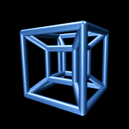
In four dimensions a rigid object can rotate in two different ways simultaneously. Such a rotation can only be represented as the sum of two simple bivectors.

In six dimensions a rigid object can rotate in three different ways simultaneously. Such a rotation can only be represented as the sum of three simple bivectors.

From Wikipedia:Bivector

The wedge product of two vectors is a bivector, but not all bivectors are wedge products of two vectors. For example, in four dimensions the bivector

$\mathbf{B} = \mathbf{e}_1 \wedge \mathbf{e}_2 + \mathbf{e}_3 \wedge \mathbf{e}_4 = \mathbf{e}_1 \mathbf{e}_2 + \mathbf{e}_3\mathbf{e}_4 = \mathbf{e}_{12} + \mathbf{e}_{34}$

cannot be written as the wedge product of two vectors. A bivector that can be written as the wedge product of two vectors is simple. In two and three dimensions all bivectors are simple, but not in four or more dimensions;

A bivector has a real square if and only if it is simple.

$\begin{align} (\mathbf{e}_{12})^2 &= e_{1212} \\ &= 1 \end{align}$

But:

$\begin{align} (\mathbf{e}_{12} + \mathbf{e}_{34})^2 &= e_{1212} + e_{1234} + e_{3412} + e_{3434} \\ &= -e_{1122} + e_{1234} + e_{1234} - e_{3344} \\ &= -1 + 2 e_{1234} -1 \\ &= 2 e_{1234} - 2 \end{align}$

Back to top

Other quadratic forms

The square of a vector is:

Failed to parse (unknown function "\begin{split}"): {\displaystyle \begin{split} \mathbf{v} \mathbf{v} &= (v_{x} {\color{blue}e_{x}} + v_{y} {\color{blue}e_{y}}) (v_{x} {\color{blue}e_{x}} + v_{y} {\color{blue}e_{y}}) \\ &= v_{x} v_{x} {\color{red}e_{x} e_{x}} + v_{x} v_{y} {\color{green}e_{x} e_{y}} + v_{y} v_{x} {\color{green}e_{y} e_{x}} + v_{y} v_{y} {\color{red}e_{y} e_{y}} \\ &= v_{x} v_{x} {\color{red}(1)} + v_{y} v_{y} {\color{red}(1)} + v_{x} v_{y} {\color{green}e_{x} e_{y}} - v_{y} v_{x} {\color{green}e_{x} e_{y}} \\ &= (v_{x} v_{x} + v_{y} v_{y}){\color{red}(1)} + (v_{x} v_{y} - v_{y} v_{x}) {\color{green}e_{xy}} \\ &= (v_{x}^2 + v_{y}^2){\color{red}(1)} + (0) {\color{green}e_{xy}} \\ &= (v_{x}^2 + v_{y}^2){\color{red}(1)} \\ &= {\color{red}\text{scalar}} \end{split} }

($v_{x}^2 + v_{y}^2$) is called the quadratic form. In this case both terms are positive but some Clifford algebras have quadratic forms with negative terms. Some have both positive and negative terms.

From Wikipedia:Clifford algebra:

Every nondegenerate quadratic form on a finite-dimensional real vector space is equivalent to the standard diagonal form:

$Q(v) = v^2 = v_1^2 + \cdots + v_p^2 - v_{p+1}^2 - \cdots - v_{p+q}^2 ,$

where n = p + q is the dimension of the vector space. The pair of integers (p, q) is called the ^*signature of the quadratic form. The real vector space with this quadratic form is often denoted R^p,q. The Clifford algebra on R^p,q is denoted Cℓ_p,q(R). The symbol Cℓ_n(R) means either Cℓ_n,0(R) or Cℓ_0,n(R) depending on whether the author prefers positive-definite or negative-definite spaces.

A standard basis^w {e_i} for R^p,q consists of n = p + q mutually orthogonal vectors, p of which square to +1 and q of which square to −1. The algebra Cℓ_p,q(R) will therefore have p vectors that square to +1 and q vectors that square to −1.

From Wikipedia:Spacetime algebra:

^*Spacetime algebra (STA) is a name for the Clifford algebra^w Cl_3,1(R), or equivalently the geometric algebra^w G(M⁴), which can be particularly closely associated with the geometry of special relativity^w and relativistic spacetime^w. See also ^*Algebra of physical space.

The spacetime algebra may be built up from an orthogonal basis of one time-like vector $\gamma_0$ and three space-like vectors, $\{\gamma_1, \gamma_2, \gamma_3\}$, with the multiplication rule

$\gamma_\mu \gamma_\nu + \gamma_\nu \gamma_\mu = 2 \eta_{\mu \nu}$

where $\eta_{\mu \nu}$ is the Minkowski metric^w with signature (− + + +).

Thus:

$\gamma_0^2 = {-1}$

$\gamma_1^2 = \gamma_2^2 = \gamma_3^2 = {+1}$

$\gamma_\mu \gamma_\nu = - \gamma_\nu \gamma_\mu$

The basis vectors $\gamma_k$ share these properties with the ^*Gamma matrices, but no explicit matrix representation need be used in STA.

Failed to parse (syntax error): {\displaystyle Cℓ_{3,0} (\mathbf{R})} :Algebra of physical space (Time = scalar)

Failed to parse (syntax error): {\displaystyle Cℓ_{3,1} (\mathbf{R})} :Spacetime algebra (Time = vector)

Failed to parse (syntax error): {\displaystyle Cℓ_{0,2} (\mathbf{R})} :Quaternions (Three quaternions = two vectors that square to -1 and one bivector that squares to -1)

Back to top

Rotors

See also: ^*Rotor (mathematics)

From Wikipedia:Geometric algebra

The inverse of a vector is:

$v^{-1} = \frac{1}{v} = \frac{v}{vv} = \frac{v}{v \cdot v + v \wedge v} = \frac{v}{v \cdot v}$

The projection of $v$ onto $a$ (or the parallel part) is

$v_{\| a} = (v \cdot a)a^{-1}$

and the rejection of $v$ from $a$ (or the orthogonal part) is

$v_{\perp a} = v - v_{\| a} = (v\wedge a)a^{-1} .$

The reflection $v'$ of a vector $v$ along a vector $a$, or equivalently across the hyperplane orthogonal to $a$, is the same as negating the component of a vector parallel to $a$. The result of the reflection will be

$v' = {-v_{\| a} + v_{\perp a}} = {-(v \cdot a)a^{-1} + (v \wedge a)a^{-1}} = {(-a \cdot v - a \wedge v)a^{-1}} = -ava^{-1}$

If a is a unit vector then $a^{-1}=\frac{a}{1} = a$ and therefore $v' = -ava$

$-ava$ is called the sandwich product which is called a double-sided product.

If we have a product of vectors $R = a_1a_2 \cdots a_r$ then we denote the reverse as

$R^\dagger = (a_1a_2\cdots a_r)^\dagger = a_r\cdots a_2 a_1.$

Any rotation is equivalent to 2 reflections.

$v'' = bv'b = bavab = RvR^\dagger$

R is called a Rotor

$R = ba = b \cdot a + b \wedge a = Scalar + Bivector = Multivector$

If a and b are unit vectors then the rotor is automatically normalised:

$RR^\dagger = R^\dagger R=1 .$

2 rotations becomes:

$R_2R_1MR_1^\dagger R_2^\dagger$

R₂R₁ represents Rotor R₁ rotated by Rotor R₂. This would be called a single-sided transformation. (R₂R₁R₂ would be double-sided.) Therefore rotors do not transform double-sided the same way that other objects do. They transform single-sided.

Back to top

Quaternions

The square root of the product of a quaternion with its conjugate is called its ^*norm:

$\lVert q \rVert = \sqrt{qq^*} = \sqrt{q^*q} = \sqrt{a^2 + b^2 + c^2 + d^2}$

A unit quaternion is a quaternion of norm one. Unit quaternions, also known as ^*versors, provide a convenient mathematical notation for representing orientations and rotations of objects in three dimensions.

From Wikipedia:Quaternions and spatial rotation

Every nonzero quaternion has a multiplicative inverse

$(a+bi+cj+dk)^{-1} = \frac{1}{a^2+b^2+c^2+d^2}\,(a-bi-cj-dk).$

Thus quaternions form a ^*division algebra.

The inverse of a unit quaternion is obtained simply by changing the sign of its imaginary components.

A ^*3-D Euclidean vector such as (2, 3, 4) or (a_x, a_y, a_z) can be rewritten as 0 + 2 i + 3 j + 4 k or 0 + a_x i + a_y j + a_z k, where i, j, k are unit vectors representing the three ^*Cartesian axes. A rotation through an angle of θ around the axis defined by a unit vector

$\vec{u} = (u_x, u_y, u_z) = 0 + u_x\mathbf{i} + u_y\mathbf{j} + u_z\mathbf{k}$

can be represented by a quaternion. This can be done using an ^*extension of Euler's formula^w:

$\mathbf{q} = e^{\frac{\theta}{2}{(0 + u_x\mathbf{i} + u_y\mathbf{j} + u_z\mathbf{k})}} = \cos \frac{\theta}{2} + (0 + u_x\mathbf{i} + u_y\mathbf{j} + u_z\mathbf{k}) \sin \frac{\theta}{2}$

It can be shown that the desired rotation can be applied to an ordinary vector $\mathbf{p} = (p_x, p_y, p_z) = 0 + p_x\mathbf{i} + p_y\mathbf{j} + p_z\mathbf{k}$ in 3-dimensional space, considered as a quaternion with a real coordinate equal to zero, by evaluating the conjugation of p by q:

$\mathbf{p'} = \mathbf{q} \mathbf{p} \mathbf{q}^{-1}$

using the ^*Hamilton product

The conjugate of a product of two quaternions is the product of the conjugates in the reverse order.

Conjugation by the product of two quaternions is the composition of conjugations by these quaternions: If p and q are unit quaternions, then rotation (conjugation) by pq is

$\mathbf{p q} \vec{v} (\mathbf{p q})^{-1} = \mathbf{p q} \vec{v} \mathbf{q}^{-1} \mathbf{p}^{-1} = \mathbf{p} (\mathbf{q} \vec{v} \mathbf{q}^{-1}) \mathbf{p}^{-1}$,

which is the same as rotating (conjugating) by q and then by p. The scalar component of the result is necessarily zero.

The imaginary part $b\mathbf{i} + c\mathbf{j} + d\mathbf{k}$ of a quaternion behaves like a vector $\vec{v} = (b,c,d)$ in three dimension vector space, and the real part a behaves like a ^*scalar in R. When quaternions are used in geometry, it is more convenient to define them as ^*a scalar plus a vector:

$a + b\mathbf{i} + c\mathbf{j} + d\mathbf{k} = a + \vec{v}.$

When multiplying the vector/imaginary parts, in place of the rules i² = j² = k² = ijk = −1 we have the quaternion multiplication rule:

$\vec{v} \vec{w} = \vec{v} \times \vec{w} - \vec{v} \cdot \vec{w},$

From these rules it follows immediately that (^*see details):

$(s + \vec{v}) (t + \vec{w}) = (s t - \vec{v} \cdot \vec{w}) + (s \vec{w} + t \vec{v} + \vec{v} \times \vec{w}).$

It is important to note, however, that the vector part of a quaternion is, in truth, an "axial" vector or "pseudovector", not an ordinary or "polar" vector.

From Wikipedia:Quaternion#Quaternions_as_the_even_part_of_Cℓ3,0(R):

the reflection of a vector r in a plane perpendicular to a unit vector w can be written:

$r^{\prime} = - w\, r\, w.$

Two reflections make a rotation by an angle twice the angle between the two reflection planes, so

$v^{\prime\prime} = \sigma_2 \sigma_1 \, v \, \sigma_1 \sigma_2$

corresponds to a rotation of 180° in the plane containing σ₁ and σ₂.

This is very similar to the corresponding quaternion formula,

$v^{\prime\prime} = -\mathbf{k}\, v\, \mathbf{k}.$

In fact, the two are identical, if we make the identification

$\mathbf{k} = \sigma_2 \sigma_1, \mathbf{i} = \sigma_3 \sigma_2, \mathbf{j} = \sigma_1 \sigma_3$

and it is straightforward to confirm that this preserves the Hamilton relations

$\mathbf{i}^2 = \mathbf{j}^2 = \mathbf{k}^2 = \mathbf{i} \mathbf{j} \mathbf{k} = -1.$

In this picture, quaternions correspond not to vectors but to bivectors^w – quantities with magnitude and orientations associated with particular 2D planes rather than 1D directions. The relation to complex numbers^w becomes clearer, too: in 2D, with two vector directions σ₁ and σ₂, there is only one bivector basis element σ₁σ₂, so only one imaginary. But in 3D, with three vector directions, there are three bivector basis elements σ₁σ₂, σ₂σ₃, σ₃σ₁, so three imaginaries.

The usefulness of quaternions for geometrical computations can be generalised to other dimensions, by identifying the quaternions as the even part Cℓ⁺_3,0(R) of the Clifford algebra^w Cℓ_3,0(R).

Back to top

Spinors

See also: ^*Bispinor

External link:An introduction to spinors

Spinors may be regarded as non-normalised rotors which transform single-sided.

Note: The (real) ^*spinors in three-dimensions are quaternions, and the action of an even-graded element on a spinor is given by ordinary quaternionic multiplication.

A spinor transforms to its negative when the space is rotated through a complete turn from 0° to 360°. This property characterizes spinors.

From Wikipedia:Orientation entanglement

In three dimensions...the ^*Lie group ^*SO(3) is not ^*simply connected. Mathematically, one can tackle this problem by exhibiting the ^*special unitary group SU(2), which is also the ^*spin group in three ^*Euclidean dimensions, as a ^*double cover of SO(3).

SU(2) is the following group,

$\mathrm{SU}(2) = \left \{ \begin{pmatrix} \alpha&-\overline{\beta}\\ \beta & \overline{\alpha} \end{pmatrix}: \ \ \alpha,\beta\in\mathbf{C}, |\alpha|^2 + |\beta|^2 = 1\right \} ~,$

where the overline denotes ^*complex conjugation.

For comparison: Using 2 × 2 complex matrices, the quaternion a + bi + cj + dk can be represented as

$\begin{bmatrix} a+bi & c+di \\ -(c-di) & a-bi \end{bmatrix}.$

If X = (x₁,x₂,x₃) is a vector in R³, then we identify X with the 2 × 2 matrix with complex entries

$X=\left(\begin{matrix}x_1&x_2-ix_3\\x_2+ix_3&-x_1\end{matrix}\right)$

Note that −det(X) gives the square of the Euclidean length of X regarded as a vector, and that X is a ^*trace-free, or better, trace-zero ^*Hermitian matrix.

The unitary group acts on X via

$X\mapsto MXM^+$

where M ∈ SU(2). Note that, since M is unitary,

$\det(MXM^+) = \det(X)$, and

$MXM^+$ is trace-zero Hermitian.

Hence SU(2) acts via rotation on the vectors X. Conversely, since any ^*change of basis which sends trace-zero Hermitian matrices to trace-zero Hermitian matrices must be unitary, it follows that every rotation also lifts to SU(2). However, each rotation is obtained from a pair of elements M and −M of SU(2). Hence SU(2) is a double-cover of SO(3). Furthermore, SU(2) is easily seen to be itself simply connected by realizing it as the group of unit ^*quaternions, a space ^*homeomorphic to the ^*3-sphere.

A unit quaternion has the cosine of half the rotation angle as its scalar part and the sine of half the rotation angle multiplying a unit vector along some rotation axis (here assumed fixed) as its pseudovector (or axial vector) part. If the initial orientation of a rigid body (with unentangled connections to its fixed surroundings) is identified with a unit quaternion having a zero pseudovector part and +1 for the scalar part, then after one complete rotation (2pi rad) the pseudovector part returns to zero and the scalar part has become -1 (entangled). After two complete rotations (4pi rad) the pseudovector part again returns to zero and the scalar part returns to +1 (unentangled), completing the cycle.

From Wikipedia:Spinors in three dimensions

The association of a spinor with a 2×2 complex ^*Hermitian matrix was formulated by Élie Cartan.

In detail, given a vector x = (x₁, x₂, x₃) of real (or complex) numbers, one can associate the complex matrix

$\vec{x} \rightarrow X \ =\left(\begin{matrix}x_3&x_1-ix_2\\x_1+ix_2&-x_3\end{matrix}\right).$

Matrices of this form have the following properties, which relate them intrinsically to the geometry of 3-space:

• det X = – (length x)².
• X ² = (length x)²I, where I is the identity matrix.
• $\frac{1}{2}(XY+YX)=({\bold x}\cdot{\bold y})I$
• $\frac{1}{2}(XY-YX)=iZ$ where Z is the matrix associated to the cross product z = x × y.
• If u is a unit vector, then −UXU is the matrix associated to the vector obtained from x by reflection in the plane orthogonal to u.
• It is an elementary fact from ^*linear algebra that any rotation in 3-space factors as a composition of two reflections. (Similarly, any orientation reversing orthogonal transformation is either a reflection or the product of three reflections.) Thus if R is a rotation, decomposing as the reflection in the plane perpendicular to a unit vector u₁ followed by the plane perpendicular to u₂, then the matrix U₂U₁XU₁U₂ represents the rotation of the vector x through R.

Having effectively encoded all of the rotational linear geometry of 3-space into a set of complex 2×2 matrices, it is natural to ask what role, if any, the 2×1 matrices (i.e., the ^*column vectors) play. Provisionally, a spinor is a column vector

$\xi=\left[\begin{matrix}\xi_1\\\xi_2\end{matrix}\right],$ with complex entries ξ₁ and ξ₂.

The space of spinors is evidently acted upon by complex 2×2 matrices. Furthermore, the product of two reflections in a given pair of unit vectors defines a 2×2 matrix whose action on euclidean vectors is a rotation, so there is an action of rotations on spinors.

Often, the first example of spinors that a student of physics encounters are the 2×1 spinors used in Pauli's theory of electron spin. The ^*Pauli matrices are a vector of three 2×2 ^*matrices that are used as ^*spin ^*operators.

Given a ^*unit vector in 3 dimensions, for example (a, b, c), one takes a ^*dot product with the Pauli spin matrices to obtain a spin matrix for spin in the direction of the unit vector.

The ^*eigenvectors of that spin matrix are the spinors for spin-1/2 oriented in the direction given by the vector.

Example: u = (0.8, -0.6, 0) is a unit vector. Dotting this with the Pauli spin matrices gives the matrix:

$S_u = (0.8,-0.6,0.0)\cdot \vec{\sigma}=0.8 \sigma_{1}-0.6\sigma_{2}+0.0\sigma_{3} = \begin{bmatrix} 0.0 & 0.8+0.6i \\ 0.8-0.6i & 0.0 \end{bmatrix}$

The eigenvectors may be found by the usual methods of ^*linear algebra, but a convenient trick is to note that a Pauli spin matrix is an ^*involutory matrix, that is, the squareof the above matrix is the identity matrix.

Thus a (matrix) solution to the eigenvector problem with eigenvalues of ±1 is simply 1 ± S_u. That is,

$S_u (1\pm S_u) = \pm 1 (1 \pm S_u)$

One can then choose either of the columns of the eigenvector matrix as the vector solution, provided that the column chosen is not zero. Taking the first column of the above, eigenvector solutions for the two eigenvalues are:

$\begin{bmatrix} 1.0+ (0.0)\\ 0.0 +(0.8-0.6i) \end{bmatrix}, \begin{bmatrix} 1.0- (0.0)\\ 0.0-(0.8-0.6i) \end{bmatrix}$

The trick used to find the eigenvectors is related to the concept of ^*ideals, that is, the matrix eigenvectors (1 ± S_u)/2 are ^*projection operators or ^*idempotents and therefore each generates an ideal in the Pauli algebra. The same trick works in any ^*Clifford algebra, in particular the ^*Dirac algebra that are discussed below. These projection operators are also seen in ^*density matrix theory where they are examples of pure density matrices.

More generally, the projection operator for spin in the (a, b, c) direction is given by

$\frac{1}{2}\begin{bmatrix}1+c&a-ib\\a+ib&1-c\end{bmatrix}$

and any non zero column can be taken as the projection operator. While the two columns appear different, one can use a² + b² + c² = 1 to show that they are multiples (possibly zero) of the same spinor.

From Wikipedia:Tensor#Spinors:

When changing from one ^*orthonormal basis (called a frame) to another by a rotation, the components of a tensor transform by that same rotation. This transformation does not depend on the path taken through the space of frames. However, the space of frames is not ^*simply connected (see ^*orientation entanglement and ^*plate trick): there are continuous paths in the space of frames with the same beginning and ending configurations that are not deformable one into the other. It is possible to attach an additional discrete invariant to each frame that incorporates this path dependence, and which turns out (locally) to have values of ±1. A ^*spinor is an object that transforms like a tensor under rotations in the frame, apart from a possible sign that is determined by the value of this discrete invariant.

Succinctly, spinors are elements of the ^*spin representation of the rotation group, while tensors are elements of its ^*tensor representations. Other ^*classical groups have tensor representations, and so also tensors that are compatible with the group, but all non-compact classical groups have infinite-dimensional unitary representations as well.

From Wikipedia:Spinor:

Quote from Elie Cartan: The Theory of Spinors, Hermann, Paris, 1966: "Spinors...provide a linear representation of the group of rotations in a space with any number $n$ of dimensions, each spinor having $2^\nu$ components where $n = 2\nu+1$ or $2\nu$." The star (*) refers to Cartan 1913.

(Note: $\nu$ is the number of ^*simultaneous independent rotations an object can have in n dimensions.)

Although spinors can be defined purely as elements of a representation space of the spin group (or its Lie algebra of infinitesimal rotations), they are typically defined as elements of a vector space that carries a linear representation of the Clifford algebra. The Clifford algebra is an associative algebra that can be constructed from Euclidean space and its inner product in a basis independent way. Both the spin group and its Lie algebra are embedded inside the Clifford algebra in a natural way, and in applications the Clifford algebra is often the easiest to work with. After choosing an orthonormal basis of Euclidean space, a representation of the Clifford algebra is generated by gamma matrices, matrices that satisfy a set of canonical anti-commutation relations. The spinors are the column vectors on which these matrices act. In three Euclidean dimensions, for instance, the Pauli spin matrices are a set of gamma matrices, and the two-component complex column vectors on which these matrices act are spinors. However, the particular matrix representation of the Clifford algebra, hence what precisely constitutes a "column vector" (or spinor), involves the choice of basis and gamma matrices in an essential way. As a representation of the spin group, this realization of spinors as (complex) column vectors will either be irreducible if the dimension is odd, or it will decompose into a pair of so-called "half-spin" or Weyl representations if the dimension is even.

In three Euclidean dimensions, for instance, spinors can be constructed by making a choice of Pauli spin matrices corresponding to (angular momenta about) the three coordinate axes. These are 2×2 matrices with complex entries, and the two-component complex column vectors on which these matrices act by matrix multiplication are the spinors. In this case, the spin group is isomorphic to the group of 2×2 unitary matrices with determinant one, which naturally sits inside the matrix algebra. This group acts by conjugation on the real vector space spanned by the Pauli matrices themselves, realizing it as a group of rotations among them, but it also acts on the column vectors (that is, the spinors).

From Wikipedia:Spinor:

In the 1920s physicists discovered that spinors are essential to describe the intrinsic angular momentum, or "spin", of the electron and other subatomic particles. More precisely, it is the fermions of spin-1/2 that are described by spinors, which is true both in the relativistic and non-relativistic theory. The wavefunction of the non-relativistic electron has values in 2 component spinors transforming under three-dimensional infinitesimal rotations. The relativistic ^*Dirac equation for the electron is an equation for 4 component spinors transforming under infinitesimal Lorentz transformations for which a substantially similar theory of spinors exists.

Back to top

Next section: Intermediate mathematics/Functions

 

See also

• Introductory mathematics
• Advanced mathematics
• ^*Impostor syndrome
• List of free mathematics books

External links

• MIT open courseware
• Cheat sheets
• http://mathinsight.org
• https://math.stackexchange.com
• https://www.eng.famu.fsu.edu/~dommelen/quantum/style_a/IV._Supplementary_Informati.html
• http://www.sosmath.com
• https://webhome.phy.duke.edu/~rgb/Class/intro_math_review/intro_math_review/node1.html
• Wikiversity:Mathematics
• w:c:4chan-science:Mathematics